import sys
import modal

print("Python:", sys.version.split()[0])
print("Modal:", modal.__version__)
Python: 3.12.13
Modal: 1.5.5
This article follows four experiments from my interactive SolveIt dialogue. The code and saved outputs are included below, so you can follow the results without running a GPU.
To run the experiments yourself, use the linked dialogue or download the notebook and setup files. You will need an authenticated Modal account for GPU inference and checkpoint storage. The checkpoint is about 10.36 GB and stays on Modal. The local notebook needs Python 3.12 and the packages in pyproject.toml. GPU usage and storage use your Modal account allowance.
Recently, I’ve been exploring how JEPA world models work in general. Today, I’m taking a closer look at I-JEPA, a method for learning useful image representations without category labels.
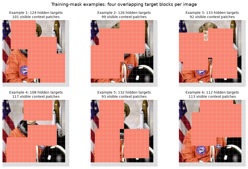
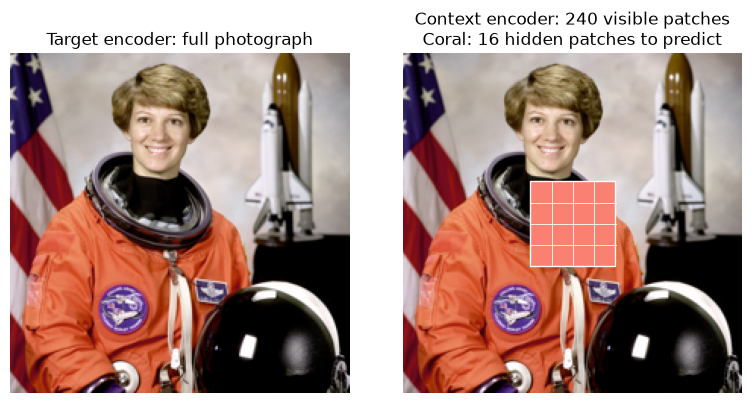
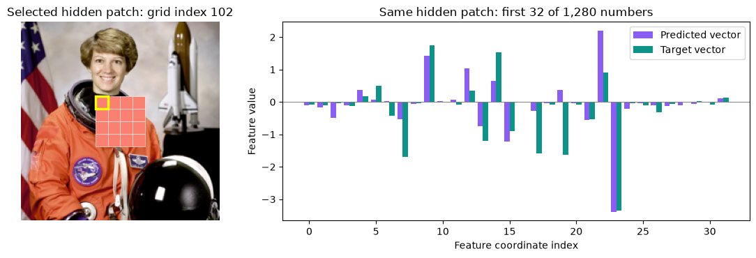
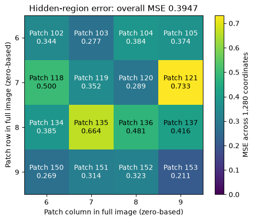
We’ll inspect the model representations it produces and examine how it learns to predict features of hidden image regions during training, using only the visible parts of the image. These predictions are vectors of learned features, rather than reconstructed pixels.
Which I-JEPA are we using? I-JEPA is a learning method with several released model variants. Here we use Meta’s I-JEPA ViT-H/14, trained on ImageNet-1K for 300 epochs: checkpoint IN1K-vit.h.14-300e.pth.tar. “ViT-H” means Vision Transformer, Huge; “/14” means 14 × 14-pixel patches.
| Detail | Our model |
|---|---|
| Encoder size | About 630 million parameters per encoder |
| Encoder structure | 32 transformer blocks |
| Input | 224 × 224 RGB image |
| Encoder output | 256 patch vectors, each with 1,280 coordinates |
| Full checkpoint download | 10.36 GB, stored on Modal |
All pretrained I-JEPA weights stay fixed throughout these experiments. In Experiment 4, we train only a new, small classifier on the encoder’s frozen features. The original training used a context encoder, a smaller predictor and a target encoder.
Our first experiment uses just the target encoder to inspect image representations. Later, we will use the context encoder and predictor to predict hidden-region representations, and the target encoder to provide a comparison. Inference can therefore involve different components, depending on the experiment.
We run I-JEPA inference on a Modal GPU and inspect the results in SolveIt. The final classifier trains on the SolveIt CPU.
Specifically we’ll focus on these main tasks:
Let’s check we can connect to the Modal servers. We first import the local Python libraries and do a version check.
import sys
import modal
print("Python:", sys.version.split()[0])
print("Modal:", modal.__version__)Python: 3.12.13
Modal: 1.5.5Next we define a small Python function remotely on Modal and display its reply here in SolveIt. This first test checks the connection using a CPU only. A successful greeting confirms authentication, remote execution and the return trip. It does not test a GPU or run I-JEPA.
app = modal.App("jepa-module-2-hello")
image = modal.Image.debian_slim(python_version="3.12")

@app.function(image=image, serialized=True, timeout=60)
def hello():
    # This function body runs on Modal.
    return "Hello from Modal!"

# Start a temporary Modal app, then bring its reply back to SolveIt.
with app.run():
    reply = hello.remote()

print(reply)
Hello from Modal!We now request an NVIDIA A10G GPU on Modal. Using PyTorch we create the tensor [1., 2., 3.] on that GPU and square each number. We expect the tensor [1.0, 4.0, 9.0] as the result.
Also, returning the device name and result checks both GPU access and actual GPU computation. The first call also builds the remote Python environment.
gpu_image = modal.Image.debian_slim(python_version="3.12").pip_install("torch==2.6.0")

@app.function(image=gpu_image, gpu="A10G", serialized=True, timeout=120)
def gpu_test():
    import torch
    x = torch.tensor([1., 2., 3.], device="cuda")
    return {"gpu": torch.cuda.get_device_name(),
            "device": str(x.device), "squares": x.square().cpu().tolist()}

with app.run():
    gpu_result = gpu_test.remote()

print(gpu_result)
{'gpu': 'NVIDIA A10', 'device': 'cuda:0', 'squares': [1.0, 4.0, 9.0]}Now we can run the pretrained target encoder from Meta’s I-JEPA ViT-H/14 checkpoint on one image input. This is a 224 × 224 RGB image. The encoder divides this image into a 16 × 16 grid of small, non-overlapping squares called patches: 256 patches in total, each measuring 14 × 14 pixels. It outputs one learned vector of 1,280 numbers for each patch.
For this first step, the whole image is visible. We are only encoding the photograph. The predictor, hidden regions and prediction error come later. The weights stay fixed from the training process. The checkpoint is downloaded into a persistent Modal Volume, not SolveIt.
The next code message defines jepa_image, extending the Modal container image we created earlier with image-processing packages and the official I-JEPA source code. It also names a persistent storage volume, weights_volume, and creates jepa_app to group our remote functions. The code only describes the setup at this stage. It does not download the checkpoint or run the encoder.
# These packages and source files are installed on Modal.
jepa_image = (gpu_image.pip_install("numpy==1.26.4", "pillow", "scikit-image")
              .apt_install("git")
              .run_commands("git clone --depth 1 https://github.com/facebookresearch/ijepa.git /opt/ijepa")
              .env({"PYTHONPATH": "/opt/ijepa"}))
weights_volume = modal.Volume.from_name("jepa-module-2-weights", create_if_missing=True)
jepa_app = modal.App("jepa-module-2-encoder")
Download or reuse the checkpoint.
Now we define prepare_weights, then call it with .remote(). The function runs on a Modal CPU and checks whether the checkpoint file is already saved under /weights in our persistent Modal Volume. If it is there, we use that saved copy instead of downloading the 10.36 GB file again.
If the file is missing, we download it with a temporary name ending in .partial. After the download finishes, the code checks that its size matches the expected number of bytes. Only then does it give the file its final checkpoint name. This prevents an interrupted download from being mistaken for a finished checkpoint on the next run.
The final print runs in SolveIt and shows the file size and storage location. No GPU or encoder is used in this step.
@jepa_app.function(image=image, volumes={"/weights": weights_volume},
                   serialized=True, timeout=900)
def prepare_weights():
    from pathlib import Path
    import urllib.request, shutil
    path = Path("/weights/IN1K-vit.h.14-300e.pth.tar")
    if not path.exists():
        url = "https://dl.fbaipublicfiles.com/ijepa/IN1K-vit.h.14-300e.pth.tar"
        with urllib.request.urlopen(url, timeout=120) as response:
            with path.with_suffix(".partial").open("wb") as destination:
                shutil.copyfileobj(response, destination, length=1024 * 1024)
        assert path.with_suffix(".partial").stat().st_size == 10358004345
        path.with_suffix(".partial").rename(path)
    return {"checkpoint_bytes": path.stat().st_size, "stored_on": "Modal Volume"}

with jepa_app.run():
    download_result = prepare_weights.remote()

print(download_result)
{'checkpoint_bytes': 10358004345, 'stored_on': 'Modal Volume'}Next we define the load_encoder function. It doesn’t load the model yet. Our Modal GPU function will call it later.
When called on Modal, it first reads the checkpoint into CPU memory (map_location="cpu"), extracts the target encoder weights and checks they match the architecture (strict=True). It then selects evaluation mode, disables weight gradients and moves the encoder to the GPU (.to("cuda")). The CPU loading happens on Modal, not in SolveIt.
def load_encoder():
    import torch
    from src.models.vision_transformer import vit_huge

    checkpoint = torch.load("/weights/IN1K-vit.h.14-300e.pth.tar",
                            map_location="cpu", weights_only=False)
    weights = {k.removeprefix("module."): v
               for k, v in checkpoint["target_encoder"].items()}
    encoder = vit_huge(patch_size=14, img_size=[224])
    encoder.load_state_dict(weights, strict=True)
    return encoder.eval().requires_grad_(False).to("cuda")
Prepare the photograph.
The code below defines our shared image preparation helper. It takes scikit-image’s bundled 512 × 512 astronaut photograph and resizes it to 224 × 224 pixels because the pretrained I-JEPA encoder configuration we use expects that size, with three colour channels (RGB). It then scales RGB values from 0–255 to 0–1. With 14 × 14-pixel patches, this gives a 16 × 16 grid: 256 patches.
permute puts the RGB channel axis first. The fixed channel means and standard deviations normalise the input. They are not a loss or a variance penalty. unsqueeze(0) adds an image-batch axis, giving (1, 3, 224, 224), and .to(device) places that tensor on the selected device passed into the function. The image and the normalised tensor used by the encoder are both returned.
def prepare_photograph(device="cuda"):
    import numpy as np
    import torch
    from PIL import Image
    from skimage.data import astronaut

    photograph = Image.fromarray(astronaut()).resize((224, 224), Image.Resampling.BICUBIC)
    pixels = torch.from_numpy(np.array(photograph)).permute(2, 0, 1).float() / 255
    mean = torch.tensor([0.485, 0.456, 0.406])[:, None, None]
    std = torch.tensor([0.229, 0.224, 0.225])[:, None, None]
    image_tensor = ((pixels - mean) / std).unsqueeze(0)
    return photograph, image_tensor.to(device)
We can test the image helper function by calling prepare_photograph on a Modal CPU using device="cpu". Below is the 224 × 224 RGB photograph it returns, followed by the shape of its normalised tensor.
The small wrapper function preview_photograph only sends the picture and tensor shape back to SolveIt. All preprocessing stays in prepare_photograph. Later, the encoder experiment calls that helper with its default device="cuda" to put the tensor on the GPU.
@jepa_app.function(image=jepa_image, serialized=True, timeout=120)
def preview_photograph():
    import io
    photograph, image_tensor = prepare_photograph(device="cpu")
    buffer = io.BytesIO()
    photograph.save(buffer, format="PNG")
    return buffer.getvalue(), tuple(image_tensor.shape)

with jepa_app.run():
    photograph_png, tensor_shape = preview_photograph.remote()

from IPython.display import Image, display
display(Image(data=photograph_png))
print("Normalised tensor shape:", tensor_shape)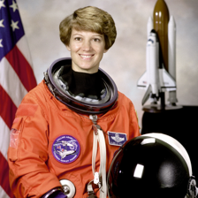
Normalised tensor shape: (1, 3, 224, 224)Our Modal function requests an A10G GPU, 32 GiB of CPU memory for loading the model checkpoint, and access to the saved weights. The following code defines encode_photograph, which we’ll use in the next step.
This is what happens when it’s called:
| Input | Computation on Modal | Output returned to SolveIt |
|---|---|---|
| 🟦 Prepared photograph → | 🟪 Target encoder on GPU → | 🟩 256 patch vectors |
| 1 × 3 × 224 × 224 | Loads its weights from the saved checkpoint | 1,280 numbers per vector |
Inside the function, we load the encoder and prepare the photograph using the helper functions previously defined. encoder(image_tensor) then computes the representations on the GPU. torch.inference_mode() disables gradient tracking, and the assertion checks for invalid numbers.
Finally, we return a small PNG preview, the input shape and the representation values to SolveIt. In the following run, we display that preview and print the input and output shapes. The checkpoint and encoder weights stay on Modal. The weights remain fixed throughout inference.
@jepa_app.function(image=jepa_image, gpu="A10G", memory=32768,
                   volumes={"/weights": weights_volume}, serialized=True, timeout=600)
def encode_photograph():
    import io, torch
    encoder = load_encoder()
    photograph, image_tensor = prepare_photograph()
    with torch.inference_mode():
        representations = encoder(image_tensor)
    assert torch.isfinite(representations).all()
    preview = io.BytesIO()
    photograph.save(preview, format="PNG")
    return {"image_png": preview.getvalue(),
            "input_shape": list(image_tensor.shape),
            "representations": representations.cpu().tolist()}
Run the experiment.
encode_photograph.remote() now executes the GPU function on Modal and waits for its result. Back in SolveIt, we display the returned photograph, store the representation values in a NumPy array and print the input and output shapes.
Below is the 224 × 224 input photograph. The printed shapes describe the encoder’s input tensor, (1, 3, 224, 224), and its output representations, (1, 256, 1280).
with jepa_app.run():
    encoded = encode_photograph.remote()

from IPython.display import Image, display
display(Image(data=encoded["image_png"]))

import numpy as np
representations = np.array(encoded["representations"])
print("Input [images, RGB channels, height, width]:", encoded["input_shape"])
print("Output [images, patches, coordinates]:", representations.shape)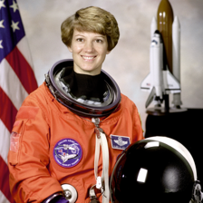
Input [images, RGB channels, height, width]: [1, 3, 224, 224]
Output [images, patches, coordinates]: (1, 256, 1280)The output axes are image, patch, feature coordinate. (1, 256, 1280) means one image, 256 patches and 1,280 numbers per patch vector. A feature coordinate is one number in that vector, rather than an x/y position in the photograph.
The code below plots the results from Modal. The left plot displays the input photograph with its top-left 14 × 14 patch outlined in red. The right plot shows the first 16 feature coordinates of that patch’s output vector, selected by representations[0, 0, :16]. These are learned features, not RGB values or named object probabilities. Because the encoder lets patches exchange information, this vector can depend on the rest of the visible image too.
import io
import matplotlib.pyplot as plt
from PIL import Image
from matplotlib.patches import Rectangle

fig, axes = plt.subplots(1, 2, figsize=(10, 4))
axes[0].imshow(Image.open(io.BytesIO(encoded["image_png"])))
axes[0].add_patch(Rectangle((-0.5, -0.5), 14, 14, fill=False, edgecolor="red", linewidth=2))
axes[0].set_title("Input photograph: patch 0 outlined")
axes[0].axis("off")
axes[1].bar(range(16), representations[0, 0, :16], color="teal")
axes[1].axhline(0, color="grey", linewidth=0.8)
axes[1].set(xlabel="Coordinate index", ylabel="Feature value",
            title="Patch 0: first 16 of 1,280 coordinates")
plt.tight_layout()
plt.show()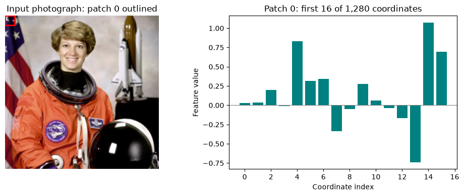
The pretrained target encoder turned one image, shaped (1, 3, 224, 224), into representations shaped (1, 256, 1280). That is 256 patch vectors, each with 1,280 coordinates. The bars show only 16 coordinates from the first patch vector.
This verifies that the real pretrained encoder runs on Modal and returns its representations to SolveIt. The plot alone does not tell us what each coordinate means or how well the model predicts hidden regions. Our next step is to introduce those hidden regions and the predictor.
In Experiment 2, we hid the astronaut’s 16 central patches and predicted their representations from the other 240 astronaut patches. We now keep those 16 astronaut target representations fixed, but make new predictions using the 240 visible patches from each of 10 other photographs. We then test whether these predictions are closer to or farther from the astronaut targets than the prediction made from the astronaut’s own visible patches.
Keeping the astronaut targets fixed is deliberate. This is a mismatched-context test: we are asking whether the astronaut’s visible regions provide more useful information for predicting its hidden-region representations than visible regions from other photographs. This is a small inference experiment with no training, so its conclusion applies only to this target photograph and the contexts tested.
We’ll select one photograph from each of ten classes with a fixed seed, before examining the errors. We use the test split of Mini-ImageNet, which contains 5,000 original ImageNet-1K validation images: 50 from each of 100 classes. These images are separate from the ImageNet training split used to pretrain I-JEPA. Hugging Face’s rows API lets us fetch only the ten selected images. We convert each to RGB and resize it to 224 × 224 in SolveIt, without running either encoder.
The resized photographs are stored in comparison_photos, and comparison_labels holds their category names for plot titles. Those labels are only for us to read; they are not given to I-JEPA.
import io, time, httpx
from PIL import Image as PILImage

comparison_row_ids = [297, 376, 431, 716, 960, 1383, 1524, 1881, 4654, 4901]
comparison_labels = ["toucan", "jellyfish", "nematode", "golden retriever",
                     "French bulldog", "lion", "rhinoceros beetle", "barrel", "trifle", "bolete"]

def fetch_image(client, row_id, attempts=5):
    params = {"dataset": "timm/mini-imagenet", "config": "default",
              "split": "test", "offset": row_id, "length": 1}
    for attempt in range(attempts):
        try:
            response = client.get("https://datasets-server.huggingface.co/rows", params=params)
            response.raise_for_status()
            row = response.json()["rows"][0]["row"]

            response = client.get(row["image"]["src"])
            response.raise_for_status()
            return PILImage.open(io.BytesIO(response.content)).convert("RGB").resize((224, 224))
        except (httpx.HTTPError, ValueError, KeyError, IndexError, OSError) as error:
            if attempt == attempts - 1:
                raise RuntimeError(f"Failed to fetch Mini-ImageNet row {row_id}") from error
            time.sleep(2 ** attempt)

with httpx.Client(timeout=30, follow_redirects=True) as client:
    comparison_photos = [fetch_image(client, row_id) for row_id in comparison_row_ids]

print(f"Downloaded {len(comparison_photos)} images:")
for row_id, class_name, image in zip(comparison_row_ids, comparison_labels, comparison_photos):
    print(f"{class_name}: row {row_id}, size={image.size}, mode={image.mode}")
Downloaded 10 images:
toucan: row 297, size=(224, 224), mode=RGB
jellyfish: row 376, size=(224, 224), mode=RGB
nematode: row 431, size=(224, 224), mode=RGB
golden retriever: row 716, size=(224, 224), mode=RGB
French bulldog: row 960, size=(224, 224), mode=RGB
lion: row 1383, size=(224, 224), mode=RGB
rhinoceros beetle: row 1524, size=(224, 224), mode=RGB
barrel: row 1881, size=(224, 224), mode=RGB
trifle: row 4654, size=(224, 224), mode=RGB
bolete: row 4901, size=(224, 224), mode=RGBHere’s what the images look like.
import matplotlib.pyplot as plt

comparison_records = []
for row_id, name in zip(comparison_row_ids, class_names):
    params = {"dataset": "timm/mini-imagenet", "config": "default", "split": "test", "offset": row_id, "length": 1}
    row = httpx.get("https://datasets-server.huggingface.co/rows", params=params, timeout=30).json()["rows"][0]["row"]
    data = httpx.get(row["image"]["src"], timeout=30).content
    original = PILImage.open(io.BytesIO(data)).convert("RGB")
    comparison_records.append({"row_id": row_id, "name": name, "original_size": original.size,
                               "download_bytes": len(data), "image": original.resize((224, 224))})

comparison_images = [record["image"] for record in comparison_records]
fig, axes = plt.subplots(2, 5, figsize=(10, 4))
for ax, record in zip(axes.flat, comparison_records):
    ax.imshow(record["image"])
    ax.set_title(record["name"])
    ax.axis("off")
plt.tight_layout()
plt.show()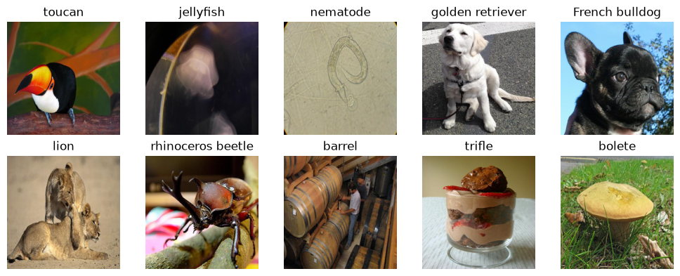
What will the context encoder see?
Each picture below shows the 240 visible patches from one comparison photograph. The coral block marks the same 16 hidden positions used in Experiment 2. It is a drawing on the plot only. The model will omit those patches, rather than receive coral pixels.
Later, the predictor will produce 16 vectors from each of these visible contexts. Every prediction will be scored against our saved astronaut target vectors, not against the hidden content of the photograph shown here. We have not calculated any new predictions yet.
import matplotlib.pyplot as plt
from matplotlib.patches import Rectangle

# Recreate the same mask so this preview also works after a session restart.
target_indices = [r*16 + c for r in range(6, 10) for c in range(6, 10)]
context_indices = [i for i in range(256) if i not in target_indices]

fig, axes = plt.subplots(2, 5, figsize=(12, 5.5))
for number, (ax, photo, label) in enumerate(zip(axes.flat, comparison_photos, comparison_labels), 1):
    ax.imshow(photo)
    # Use the existing hidden-patch indices, so this matches Experiment 2 exactly.
    for patch_id in target_indices:
        row, column = divmod(patch_id, 16)
        ax.add_patch(Rectangle((column*14-0.5, row*14-0.5), 14, 14,
                               facecolor="salmon", edgecolor="white", lw=0.4))
    # Show the complete 16 × 16 patch grid, including the visible context.
    for edge in range(0, 225, 14):
        ax.axhline(edge - 0.5, color="white", lw=0.35, alpha=0.65)
        ax.axvline(edge - 0.5, color="white", lw=0.35, alpha=0.65)
    ax.set_title(f"{number}. {label}", fontsize=10)
    ax.axis("off")
fig.suptitle("Ten alternative visible contexts: same 16 hidden positions", fontsize=13)
plt.tight_layout()
plt.show()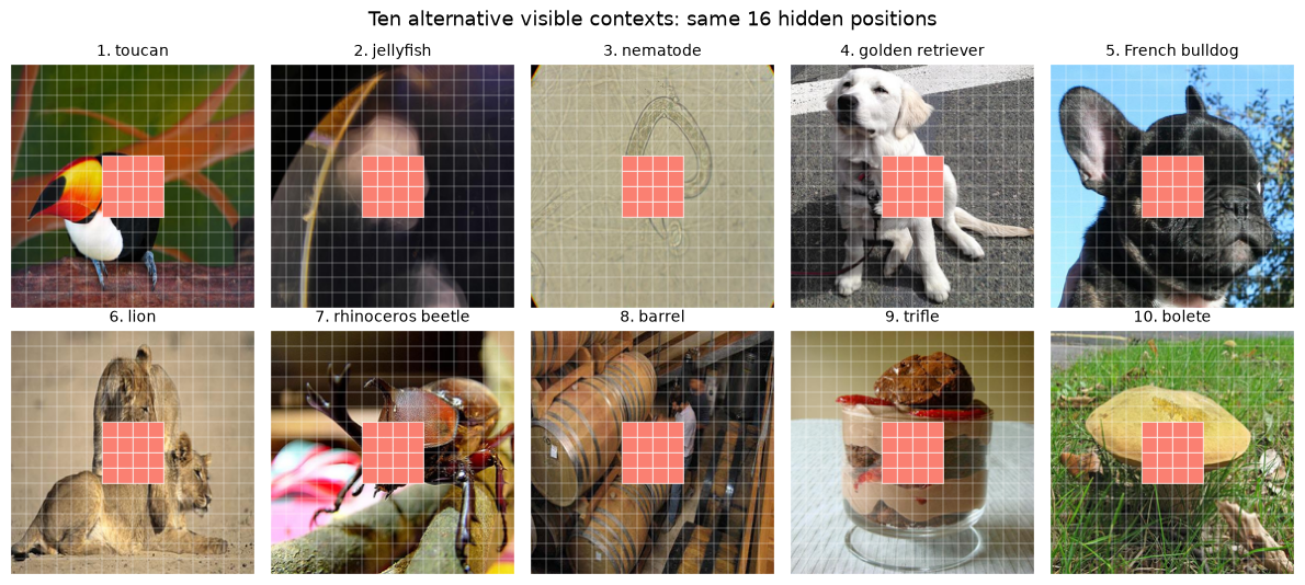
Each new photograph will produce 16 predicted vectors, each containing 1,280 numbers. We compare them with the astronaut’s 16 normalised target vectors from Experiment 2, in exactly the same patch order. These targets act like numerical labels for this comparison.
First we preserve the astronaut targets and its original prediction. If the SolveIt session has restarted, we restore that reference from a small saved results file or rerun the astronaut calculation once with the same checkpoint and mask. We never create targets from the ten comparison photographs.
import modal

# Recreate the same Modal setup if this SolveIt session was restarted.
if "jepa_app" not in globals():
    gpu_image = modal.Image.debian_slim(python_version="3.12").pip_install("torch==2.6.0")
    jepa_image = (gpu_image.pip_install("numpy==1.26.4", "pillow", "scikit-image")
                  .apt_install("git")
                  .run_commands("git clone --depth 1 https://github.com/facebookresearch/ijepa.git /opt/ijepa")
                  .env({"PYTHONPATH": "/opt/ijepa"}))
    weights_volume = modal.Volume.from_name("jepa-module-2-weights", create_if_missing=False)
    jepa_app = modal.App("jepa-module-2-encoder")
print("Modal setup ready. The pretrained checkpoint stays in its existing Modal volume.")
Modal setup ready. The pretrained checkpoint stays in its existing Modal volume.After a session restart, rerun the earlier definition messages for load_jepa_networks, prepare_photograph and predict_hidden_region. They only define functions. The next message restores the astronaut arrays and saves them in ijepa_astronaut_reference.npz beside this dialogue. Future runs can load that small file without repeating the astronaut GPU calculation.
from pathlib import Path
import numpy as np

reference_path = Path("ijepa_astronaut_reference.npz")
if reference_path.exists():
    with np.load(reference_path) as saved:
        assert np.array_equal(saved["patch_indices"], target_indices)
        astronaut_targets = saved["targets"].copy()
        astronaut_predictions = saved["predictions"].copy()
else:
    if "hidden_result" not in globals():
        print("Restoring the astronaut reference on Modal…", flush=True)
        with jepa_app.run():
            hidden_result = predict_hidden_region.remote(context_indices, target_indices)
    astronaut_targets = np.array(hidden_result["targets"])
    astronaut_predictions = np.array(hidden_result["predictions"])
    np.savez_compressed(reference_path, targets=astronaut_targets,
                        predictions=astronaut_predictions, patch_indices=target_indices)

assert astronaut_targets.shape == astronaut_predictions.shape == (1, 16, 1280)
assert np.isfinite(astronaut_targets).all() and np.isfinite(astronaut_predictions).all()
astronaut_mse = ((astronaut_predictions - astronaut_targets) ** 2).mean()
print(f"Astronaut reference ready: {astronaut_targets.shape}, baseline MSE {astronaut_mse:.4f}")
Astronaut reference ready: (1, 16, 1280), baseline MSE 0.3947We send the ten resized photographs to Modal as PNG data. The helper below converts each photograph to the same normalised input tensor used in Experiment 2: RGB values divided by 255, followed by the same channel means and standard deviations. It does not resize the photograph again.
On the GPU, the context encoder processes only the 240 visible patch positions. The predictor then produces 16 vectors in target_indices order. We keep its output unchanged, with no extra vector normalisation. All weights remain fixed.
def comparison_image_tensor(png_bytes):
    import io, numpy as np, torch
    from PIL import Image

    photograph = Image.open(io.BytesIO(png_bytes)).convert("RGB")
    assert photograph.size == (224, 224)
    pixels = torch.from_numpy(np.array(photograph)).permute(2, 0, 1).float() / 255
    mean = torch.tensor([0.485, 0.456, 0.406])[:, None, None]
    std = torch.tensor([0.229, 0.224, 0.225])[:, None, None]
    return ((pixels - mean) / std).unsqueeze(0).to("cuda")
The next function reuses load_jepa_networks. That helper loads all three networks, so we immediately release the unused target encoder. None of the ten new photographs goes through the target encoder. We process one photograph at a time to keep GPU memory use modest, then return the ten sets of predictions in the same order as the preview.
@jepa_app.function(image=jepa_image, gpu="A10G", memory=32768,
                   volumes={"/weights": weights_volume}, serialized=True, timeout=600)
def predict_comparison_photos(photo_pngs, context_indices, target_indices):
    import torch

    context_encoder, predictor, unused_target = load_jepa_networks()
    del unused_target
    context_mask = torch.tensor([context_indices], dtype=torch.long, device="cuda")
    target_mask = torch.tensor([target_indices], dtype=torch.long, device="cuda")
    predictions = []
    with torch.inference_mode():
        for photo_png in photo_pngs:
            image_tensor = comparison_image_tensor(photo_png)
            visible_vectors = context_encoder(image_tensor, masks=[context_mask])
            predicted = predictor(visible_vectors, [context_mask], [target_mask])
            assert predicted.shape == (1, len(target_indices), 1280)
            assert torch.isfinite(predicted).all()
            predictions.append(predicted[0].cpu().tolist())
    return {"predictions": predictions, "patch_indices": target_indices,
            "gpu": torch.cuda.get_device_name()}
Now we call the GPU function. Its returned array will have shape (10, 16, 1280): ten context photographs, sixteen hidden patch positions and 1,280 coordinates per vector. The PNGs contain the original resized pictures. The coral blocks and grid lines exist only in our preview plot.
We save the returned vectors, astronaut reference, patch positions and photograph identifiers in a small results file. The next error calculations and plots run in SolveIt without another GPU call.
import io

comparison_pngs = []
for photograph in comparison_photos:
    buffer = io.BytesIO()
    photograph.save(buffer, format="PNG")
    comparison_pngs.append(buffer.getvalue())

print("Predicting ten photographs on Modal…", flush=True)
with jepa_app.run():
    comparison_result = predict_comparison_photos.remote(comparison_pngs, context_indices, target_indices)
comparison_predictions = np.array(comparison_result["predictions"])
assert comparison_predictions.shape == (10, 16, 1280)
assert comparison_result["patch_indices"] == target_indices
np.savez_compressed("ijepa_context_comparison.npz", predictions=comparison_predictions,
                    astronaut_targets=astronaut_targets, astronaut_predictions=astronaut_predictions,
                    patch_indices=target_indices, row_ids=comparison_row_ids, labels=comparison_labels)
print("GPU:", comparison_result["gpu"])
print("Predictions [photograph, hidden patch, coordinate]:", comparison_predictions.shape)
print("Saved results to ijepa_context_comparison.npz")
Predicting ten photographs on Modal…
GPU: NVIDIA A10
Predictions [photograph, hidden patch, coordinate]: (10, 16, 1280)
Saved results to ijepa_context_comparison.npzFor example, comparison_predictions[0, 0, 5] is coordinate 5 of the first hidden-patch prediction made from the first comparison photograph. We compare it with astronaut_targets[0, 0, 5], the same coordinate and patch position in the astronaut reference.
We subtract, square and average all 16 × 1,280 differences per photograph to obtain ten MSE scores. NumPy reuses the single astronaut target array for each photograph automatically. This is called broadcasting. A score below the astronaut baseline means that alternative context matched these astronaut targets more closely. A higher score means it matched them less closely.
import pandas as pd

assert comparison_predictions.shape == (10, 16, 1280)
assert astronaut_targets.shape == (1, 16, 1280)
comparison_squared_errors = (comparison_predictions - astronaut_targets) ** 2
comparison_mse = comparison_squared_errors.mean(axis=(1, 2))

comparison_scores = pd.DataFrame({
    "Visible context": comparison_labels,
    "MSE against astronaut targets": comparison_mse,
    "MSE minus astronaut baseline": comparison_mse - astronaut_mse,
})
print(f"Astronaut context baseline: {astronaut_mse:.4f}")
print("Each score averages 20,480 coordinate comparisons.")
display(comparison_scores.round(4))
print(f"Lower error than astronaut context: {int((comparison_mse < astronaut_mse).sum())}/10")
print(f"Higher error than astronaut context: {int((comparison_mse > astronaut_mse).sum())}/10")
Astronaut context baseline: 0.3947
Each score averages 20,480 coordinate comparisons.| Visible context | MSE against astronaut targets | MSE minus astronaut baseline | |
|---|---|---|---|
| 0 | toucan | 1.4748 | 1.0801 |
| 1 | jellyfish | 1.2615 | 0.8668 |
| 2 | nematode | 1.4260 | 1.0314 |
| 3 | golden retriever | 1.3857 | 0.9911 |
| 4 | French bulldog | 1.7417 | 1.3470 |
| 5 | lion | 1.3531 | 0.9585 |
| 6 | rhinoceros beetle | 1.4000 | 1.0054 |
| 7 | barrel | 1.5440 | 1.1493 |
| 8 | trifle | 1.5236 | 1.1290 |
| 9 | bolete | 1.4948 | 1.1001 |
Lower error than astronaut context: 0/10
Higher error than astronaut context: 10/10
The MSE minus astronaut baseline table column subtracts the astronaut’s own error (0.3947) from each photograph’s error. For example, the toucan gives 1.4748 − 0.3947 = 1.0801, so its error is 1.0801 higher than the astronaut baseline.
A positive difference means higher error, a negative difference means lower error, and zero means equal error. This column expresses the same MSE relative to our baseline. It is not a separate measurement or a percentage.
Read the result visually. Every bar in the plot below is an error against the same sixteen astronaut target vectors. Teal shows the astronaut’s own visible context. Purple shows each alternative photograph’s visible context. Shorter bars mean closer matches. The dashed line marks the astronaut baseline.
import matplotlib.pyplot as plt

plot_labels = ["Astronaut (same image)"] + comparison_labels
plot_errors = np.r_[astronaut_mse, comparison_mse]
fig, ax = plt.subplots(figsize=(9, 5.5))
bars = ax.barh(plot_labels, plot_errors, color=["#0d9488"] + ["#8b5cf6"] * 10)
ax.axvline(astronaut_mse, color="#0d9488", linestyle="--", linewidth=1)
ax.bar_label(bars, fmt="%.3f", padding=5, fontsize=9)
ax.invert_yaxis()
ax.set(xlabel="Mean squared error against the fixed astronaut targets (lower is better)",
       title="Does the astronaut’s own visible context help?", xlim=(0, plot_errors.max()*1.15))
ax.spines[["top", "right"]].set_visible(False)
plt.tight_layout()
plt.show()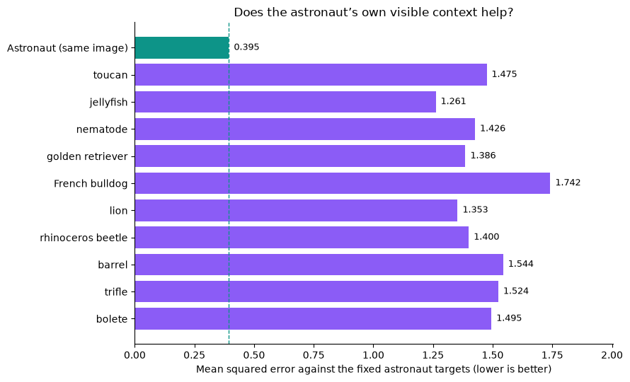
The astronaut’s own visible context gave an MSE of 0.3947. All ten alternative contexts gave higher errors, ranging from 1.2615 to 1.7417. For this photograph and hidden region, the matching visible context helped the predictor produce vectors closer to the astronaut targets.
This is evidence about one target photograph and ten alternative contexts, not a general accuracy score. The target encoder’s patch vectors also incorporate information from the full astronaut image, so this test measures agreement with those contextual representations. It does not show that the model reconstructed the hidden pixels.
We have now inspected the encoder, traced hidden-patch prediction and tested the effect of changing its visible context. Experiment 4 will put the learned representations to practical use with a small image classifier.
So far, we have inspected I-JEPA’s representations and hidden-patch predictions. Now we’ll use its learned features for a practical task: predict which of ten categories a photograph belongs to. We’ll collect labelled examples of the same ten categories used in Experiment 3, with separate training and test photographs.
The pretrained target encoder will process each full photograph on Modal, with no patches hidden. We’ll average its 256 patch vectors to obtain one vector of 1,280 numbers per photograph, then return those vectors to SolveIt. The encoder’s weights stay fixed throughout. We won’t use the context encoder or predictor in this experiment.
In SolveIt, we’ll train a small linear classifier that maps each image vector to ten class scores. Only this classifier learns from the category labels. This is called a linear probe: it tests how useful the frozen encoder’s features are for separating the categories. Finally, we’ll evaluate on photographs withheld from classifier training, inspect correct predictions and mistakes, and finally wrap up what we have learned about I-JEPA.
We will build a balanced ten-class dataset for the linear probe using the test split of timm/mini-imagenet. For each category, we need 40 new photographs: 30 for classifier training and 10 held out for testing. Across ten categories, that gives 300 training images and 100 test images.
Mini-ImageNet’s test split contains ImageNet-1K validation images, whereas this I-JEPA checkpoint was pretrained on the ImageNet-1K training split. Our probe records are therefore outside the checkpoint’s documented pretraining set. This establishes separation between the official dataset splits, but does not rule out visually similar or near-duplicate photographs across them.
Experiment 3 already used one of the 50 available validation photographs in each category. We exclude that record, leaving 49 candidates per category. A reproducible seeded selection will later assign 30 to classifier training and 10 different records to held-out testing, leaving 9 unused.
Here, training and test refer to our linear probe, not I-JEPA pretraining or Mini-ImageNet’s own split names. The following code reads row metadata for the ten Experiment 3 examples so we can identify their source labels; it does not download or encode the photographs.
import httpx
import numpy as np
import pandas as pd

TRAIN_PER_CLASS, TEST_PER_CLASS = 30, 10
PROBE_SEED = 42
probe_classes = list(comparison_labels)
source = dict(dataset="timm/mini-imagenet", config="default", split="test")

def dataset_records(endpoint, **query):
    """Read image metadata without downloading the photographs."""
    response = httpx.get(
        f"https://datasets-server.huggingface.co/{endpoint}",
        params={**source, **query}, timeout=60, follow_redirects=True)
    response.raise_for_status()
    return response.json()["rows"]

# Existing examples identify the dataset label for each of our categories.
probe_source_labels = [
    dataset_records("rows", offset=row_id, length=1)[0]["row"]["label"]
    for row_id in comparison_row_ids
]
assert len(set(probe_source_labels)) == 10
display(pd.DataFrame({"Category": probe_classes, "Dataset label": probe_source_labels}))| Category | Dataset label | |
|---|---|---|
| 0 | toucan | 5 |
| 1 | jellyfish | 7 |
| 2 | nematode | 8 |
| 3 | golden retriever | 14 |
| 4 | French bulldog | 19 |
| 5 | lion | 27 |
| 6 | rhinoceros beetle | 30 |
| 7 | barrel | 37 |
| 8 | trifle | 93 |
| 9 | bolete | 98 |
The table maps our ten category names to Mini-ImageNet’s source labels. These numbers identify dataset classes; they are not model scores or predictions. For the linear classifier, we will later map the same categories to labels 0 through 9.
Using each source label, the next code gathers all other records from that category while excluding the exact row used in Experiment 3. At this stage it only constructs and checks the candidate pools; it does not yet choose the classifier-training and held-out records.
probe_pools = []
for row_id, source_label in zip(comparison_row_ids, probe_source_labels):
    # Read nearby records, then keep only the matching category.
    rows = dataset_records("rows", offset=max(0, row_id - 50), length=100)
    pool = [r for r in rows
            if r["row"]["label"] == source_label
            and r["row_idx"] not in comparison_row_ids]
    probe_pools.append(pool)

print("Confirmed available records per category:", [len(pool) for pool in probe_pools])
Confirmed available records per category: [49, 49, 49, 49, 49, 49, 49, 49, 49, 49]The check confirms 49 available candidates per category after excluding the ten Experiment 3 records. The next selection step will reproducibly shuffle each pool, choose 30 records for classifier training and 10 for held-out testing, and leave 9 unused.
We will verify that all 400 selected row IDs are unique, that the training and held-out sets do not overlap, and that none reuses an Experiment 3 row. The 100 held-out photographs will not be used to fit the linear classifier; they will be used only for evaluation after fitting.
Each category begins with 49 eligible records: its 50 Mini-ImageNet test/Imagenet-1K validation records, minus the exact record used in Experiment 3.
For each category, rng.permutation creates a reproducibly shuffled ordering of those 49 record positions. We take the first 40 positions without replacement: positions 0–29 become 30 classifier-training examples, and positions 30–39 become 10 separate held-out test examples. Positions 40–48 are unused. The test images do not come from another dataset or another pool; they are distinct records from the same 49-record category pool.
The code then checks that all 400 selected row IDs are globally unique and that none equals any Experiment 3 row ID. It saves the exact selection so later steps reuse the same split.
rng = np.random.default_rng(PROBE_SEED)
probe_records = []
needed = TRAIN_PER_CLASS + TEST_PER_CLASS

for class_id, (name, pool) in enumerate(zip(probe_classes, probe_pools)):
    assert len(pool) >= needed, f"Not enough examples for {name}"
    chosen = rng.permutation(len(pool))[:needed]
    for position, index in enumerate(chosen):
        record = pool[index]
        probe_records.append({
            "row_id": record["row_idx"], "class_id": class_id, "category": name,
            "split": "train" if position < TRAIN_PER_CLASS else "test",
            "image_url": record["row"]["image"]["src"],
        })

probe_manifest = pd.DataFrame(probe_records)
assert probe_manifest.row_id.is_unique  # Also prevents train/test overlap.
assert not set(probe_manifest.row_id) & set(comparison_row_ids)
probe_manifest.to_json("ijepa_probe_manifest.json", orient="records", indent=2)
probe_counts = pd.crosstab(probe_manifest.category, probe_manifest.split)
probe_counts = probe_counts.reindex(probe_classes)[["train", "test"]]
print(f"Saved {len(probe_manifest)} records. No overlapping row IDs.")
Saved 400 records. No overlapping row IDs.The chart below shows how many photographs each category contributes. Teal is training and purple is testing. Equal counts prevent a frequent category from dominating our small evaluation. No encoder or classifier has run in this step.
import matplotlib.pyplot as plt

ax = probe_counts.plot.barh(stacked=True, color=["#0d9488", "#8b5cf6"], figsize=(8, 4))
ax.invert_yaxis()
ax.set(xlabel="Number of photographs", ylabel="", title="Our classifier data: 300 training + 100 test")
ax.legend(["Training", "Test"], loc="upper left", bbox_to_anchor=(1, 1))
for bars in ax.containers:
    ax.bar_label(bars, label_type="center", color="white")
plt.tight_layout()
plt.show()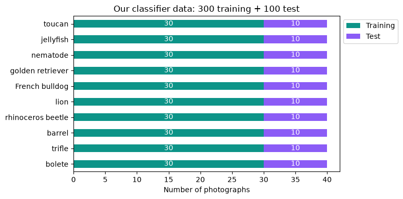
We now download the 400 selected photographs in the order recorded in probe_manifest. Each is converted to RGB and resized to 224 × 224 pixels, as in our earlier experiments. Small PNG copies are cached in SolveIt so rerunning this step reuses them. The model weights stay on Modal.
The helper below loads one photograph. If a saved image link has expired, it uses our earlier fetch_image helper to request a fresh one.
import io
from pathlib import Path
from PIL import Image
from concurrent.futures import ThreadPoolExecutor

probe_image_dir = Path("ijepa_probe_images_224")
probe_image_dir.mkdir(exist_ok=True)

def load_probe_png(record):
    path = probe_image_dir / f"test_{record.row_id}.png"
    if not path.exists():
        with httpx.Client(timeout=30, follow_redirects=True) as client:
            try:
                response = client.get(record.image_url)
                response.raise_for_status()
                photograph = Image.open(io.BytesIO(response.content)).convert("RGB")
                photograph = photograph.resize((224, 224), Image.Resampling.BICUBIC)
            except httpx.HTTPError:
                photograph = fetch_image(client, record.row_id)
        photograph.save(path, format="PNG")
    return path.read_bytes()
We load four photographs at a time to reduce download time. pool.map preserves the manifest order, so every image stays aligned with its category label and training/test assignment.
with ThreadPoolExecutor(max_workers=4) as pool:
    probe_pngs = list(pool.map(load_probe_png, probe_manifest.itertuples(index=False)))

assert len(probe_pngs) == len(probe_manifest)
print(f"Ready: {len(probe_pngs)} RGB photographs, each 224 × 224 pixels.")
print(f"Cached PNGs: {sum(map(len, probe_pngs)) / 1e6:.1f} MB")
Ready: 400 RGB photographs, each 224 × 224 pixels.
Cached PNGs: 32.6 MBA quick visual check: below is one training photograph per category, after resizing. These are actual classifier inputs. We leave the held-out photographs for the final evaluation.
preview_rows = probe_manifest.query("split == 'train'").groupby("class_id", sort=True).head(1)
fig, axes = plt.subplots(2, 5, figsize=(11, 5))
for ax, (index, record) in zip(axes.flat, preview_rows.iterrows()):
    ax.imshow(Image.open(io.BytesIO(probe_pngs[index])))
    ax.set_title(record.category, fontsize=10)
    ax.axis("off")
plt.tight_layout()
plt.show()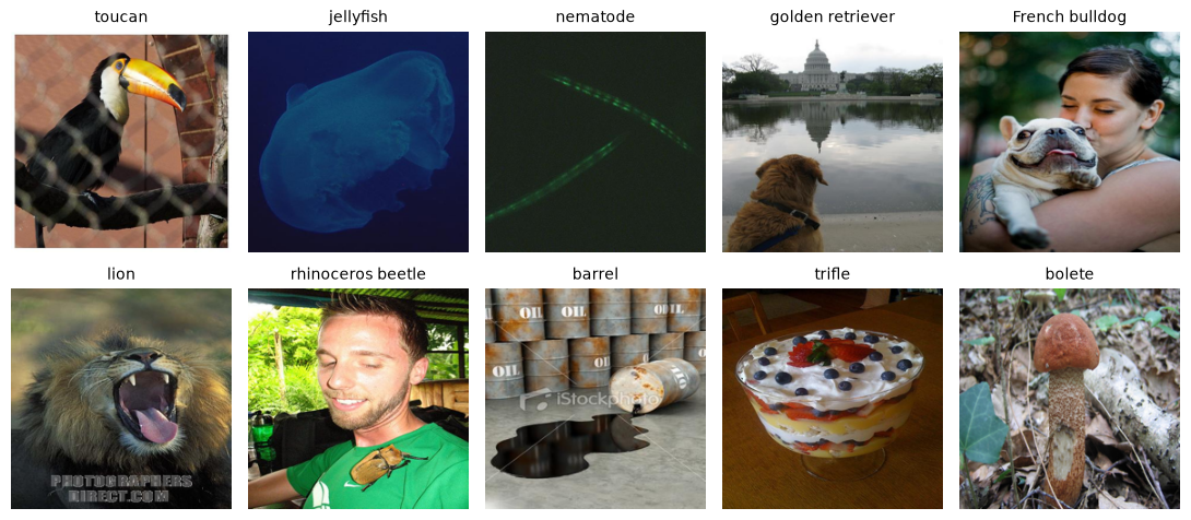
On Modal we reuse load_encoder() from Experiment 1 to load only the pretrained target encoder. We reuse comparison_image_tensor() from Experiment 3 for pixel normalisation. Despite that helper’s name, it simply prepares an image tensor.
We process eight full photographs at a time. The encoder returns (8, 256, 1280): eight images, 256 patch vectors per image, and 1,280 coordinates per vector. mean(dim=1) averages across the patches, leaving (8, 1280). The final smaller batch works the same way.
This is inference only: no masks, predictor, loss or weight updates. We use the encoder’s output directly, without the extra target normalisation used for hidden-patch prediction.
@jepa_app.function(image=jepa_image, gpu="A10G", memory=32768,
                   volumes={"/weights": weights_volume}, serialized=True, timeout=900)
def extract_probe_features(photo_pngs, batch_size=8):
    import torch

    encoder = load_encoder()  # Frozen pretrained target encoder only.
    feature_batches = []
    with torch.inference_mode():
        for start in range(0, len(photo_pngs), batch_size):
            batch = torch.cat([comparison_image_tensor(png)
                               for png in photo_pngs[start:start + batch_size]])
            patch_vectors = encoder(batch)          # [images, 256, 1280]
            image_vectors = patch_vectors.mean(dim=1)  # [images, 1280]
            assert torch.isfinite(image_vectors).all()
            feature_batches.append(image_vectors.cpu())

    return {"features": torch.cat(feature_batches).numpy(),
            "gpu": torch.cuda.get_device_name()}
Now we call the GPU function and save its returned feature array in SolveIt. A fingerprint of the image bytes, their order and this encoder recipe identifies the cache. Repeating the same experiment can load the saved features without another GPU call. The expected output is (400, 1280). The function receives photographs only, not category labels.
import hashlib

recipe = b"IN1K-vit.h.14-300e-target-meanpool-rgb224-v1"
fingerprint = hashlib.sha256(recipe + b"".join(
    hashlib.sha256(png).digest() for png in probe_pngs)).hexdigest()[:16]
feature_path = Path(f"ijepa_probe_features_{fingerprint}.npz")

if feature_path.exists():
    with np.load(feature_path) as saved:
        probe_features = saved["features"].copy()
    print("Loaded cached features.")
else:
    print("Encoding 400 photographs on Modal…", flush=True)
    with jepa_app.run():
        feature_result = extract_probe_features.remote(probe_pngs)
    probe_features = feature_result["features"]
    np.savez_compressed(feature_path, features=probe_features,
                        row_ids=probe_manifest.row_id.to_numpy())
    print("GPU:", feature_result["gpu"])

assert probe_features.shape == (len(probe_manifest), 1280)
assert np.isfinite(probe_features).all()
print("Features [photograph, coordinate]:", probe_features.shape)
print(f"Saved feature file: {feature_path.stat().st_size / 1e6:.2f} MB")
Encoding 400 photographs on Modal…
GPU: NVIDIA A10
Features [photograph, coordinate]: (400, 1280)
Saved feature file: 1.93 MBEach returned row will describe one whole photograph, in the same order as probe_manifest. For example, probe_features[0] will contain the 1,280 features for the first photograph. These values are learned image features, not class scores.
Next we’ll separate these rows using our saved training/test assignments. Only the 300 training vectors and their category labels will be used to fit the linear classifier.
train_mask = probe_manifest["split"].eq("train").to_numpy()
probe_labels = probe_manifest["class_id"].to_numpy(dtype=np.int64)

X_train, X_test = probe_features[train_mask], probe_features[~train_mask]
y_train, y_test = probe_labels[train_mask], probe_labels[~train_mask]

assert X_train.shape == (300, 1280) and X_test.shape == (100, 1280)
assert np.all(np.bincount(y_train, minlength=10) == 30)
assert np.all(np.bincount(y_test, minlength=10) == 10)
print("Training: features", X_train.shape, "labels", y_train.shape)
print("Test:     features", X_test.shape, "labels", y_test.shape)
Training: features (300, 1280) labels (300,)
Test: features (100, 1280) labels (100,)Each training photograph already has a 1,280-number feature vector from the frozen target encoder. We’ll now teach a new classifier to map that vector to ten class scores, one for each category.
Saved image vector → linear layer → ten scores → highest-scoring category
The classifier is a single linear layer with no hidden layers. Each score is a weighted sum of the 1,280 input values plus a bias. Only these 12,810 classifier parameters will learn. This is a standard linear probe. Everything in this subsection runs on SolveIt’s CPU, using only X_train and y_train.
import torch
from torch import nn

torch.manual_seed(PROBE_SEED)
train_features = torch.tensor(X_train, dtype=torch.float32, device="cpu")
train_labels = torch.tensor(y_train, dtype=torch.long, device="cpu")
classifier = nn.Linear(1280, len(probe_classes)).to("cpu")

print(classifier)
print("Trainable parameters:", sum(p.numel() for p in classifier.parameters()))
print("Device:", next(classifier.parameters()).device)
Linear(in_features=1280, out_features=10, bias=True)
Trainable parameters: 12810
Device: cpuWhat supplies the training error? The classifier outputs ten raw scores, called logits, for each photograph. CrossEntropyLoss compares those scores with the correct category in train_labels. Internally it converts scores into relative class probabilities and penalises low probability for the correct category. We pass raw scores directly to it.
We’ll use all 300 training vectors in each update, for 200 updates. Adam adjusts only the classifier’s weights and biases. The learning rate is 0.01, with 0.001 weight decay to discourage large weights. These are fixed settings for our demonstration, chosen without consulting the test results.
probe_steps, probe_lr, probe_decay = 200, 0.01, 0.001
loss_fn = nn.CrossEntropyLoss()
optimizer = torch.optim.Adam(classifier.parameters(), lr=probe_lr, weight_decay=probe_decay)
training_losses = []
classifier.train()

for step in range(probe_steps):
    optimizer.zero_grad()                    # Clear previous gradients.
    scores = classifier(train_features)      # Forward: [300, 10] scores.
    loss = loss_fn(scores, train_labels)      # Compare with 300 category labels.
    assert torch.isfinite(loss)
    training_losses.append(loss.item())       # Loss before this update.
    loss.backward()                          # One backpropagation through classifier.
    optimizer.step()                         # Update classifier weights and biases.

classifier.eval()
with torch.no_grad():
    final_training_loss = loss_fn(classifier(train_features), train_labels).item()
training_losses.append(final_training_loss)
print(f"Training cross-entropy: {training_losses[0]:.4f} → {training_losses[-1]:.4f}")
print(f"Completed {probe_steps} CPU updates. The encoder weights were unchanged.")
Training cross-entropy: 2.3613 → 0.0014
Completed 200 CPU updates. The encoder weights were unchanged.The plot below tracks average training cross-entropy against the number of completed weight updates. Point 0 is before training and point 200 is after the final update. Lower loss means the classifier assigns higher probability to the correct categories on these training photographs. The curve shows cross-entropy only, not the weight-decay contribution.
Note: This is a training diagnostic, not held-out accuracy.
import matplotlib.pyplot as plt

fig, ax = plt.subplots(figsize=(8, 3.5))
ax.plot(range(len(training_losses)), training_losses, color="#0d9488", linewidth=2)
ax.set(xlabel="Completed classifier weight updates", ylabel="Training cross-entropy",
       title="Linear probe: fitting the 300 training photographs", ylim=(0, None))
ax.spines[["top", "right"]].set_visible(False)
plt.tight_layout()
plt.show()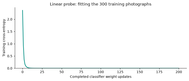
Training cross-entropy fell from 2.3613 to 0.0014. This demonstrates that the classifier can fit these training features closely, but we have not yet measured how it performs on held-out photographs.
We save the classifier weights, category order and training settings below. The target encoder stays unchanged on Modal. Next step: evaluate this fixed classifier on the 100 held-out feature vectors.
torch.save({
    "state_dict": classifier.state_dict(),
    "classes": list(probe_classes),
    "feature_cache": str(feature_path),
    "training_row_ids": probe_manifest.loc[train_mask, "row_id"].tolist(),
    "seed": PROBE_SEED, "updates": probe_steps,
    "learning_rate": probe_lr, "weight_decay": probe_decay,
    "training_losses": training_losses,
}, "ijepa_linear_probe.pt")
print("Saved trained classifier to ijepa_linear_probe.pt")
Saved trained classifier to ijepa_linear_probe.ptWe now use the 100 held-out photographs: ten per category. Their saved target-encoder vectors go through the trained classifier. For each photograph, the highest of its ten scores determines the predicted category. We compare that category with the correct label and count the matches.
This runs on SolveIt’s CPU with no training or weight updates. Uniform random guessing would average 10% accuracy across these ten categories. We keep the training settings fixed after seeing the results.
test_features = torch.tensor(X_test, dtype=torch.float32, device="cpu")
classifier.eval()
with torch.inference_mode():
    test_scores = classifier(test_features)  # [100 photographs, 10 class scores]
    test_predictions = test_scores.argmax(dim=1).numpy()

assert test_scores.shape == (100, 10) and torch.isfinite(test_scores).all()
correct = test_predictions == y_test
test_accuracy = correct.mean()
print(f"Held-out accuracy: {correct.sum()}/{len(correct)} = {test_accuracy:.0%}")
print("Uniform random guessing: 10% expected accuracy")
Held-out accuracy: 98/100 = 98%
Uniform random guessing: 10% expected accuracy98 of 100 held-out photographs were classified correctly. The chart below breaks that result down by category. Each bar counts correct predictions out of ten photographs. The dashed line marks one correct out of ten, the average expected from uniform random guessing.
correct_per_class = [int(correct[y_test == k].sum()) for k in range(len(probe_classes))]
fig, ax = plt.subplots(figsize=(8, 4))
bars = ax.barh(probe_classes, correct_per_class, color="#0d9488")
ax.bar_label(bars, labels=[f"{n}/10" for n in correct_per_class], padding=4)
ax.axvline(1, color="#d97706", linestyle="--", label="Random guessing: expected 1/10")
ax.set(xlim=(0, 11.5), xlabel="Correct predictions out of ten held-out photographs",
       title=f"Held-out classification accuracy: {test_accuracy:.0%}")
ax.invert_yaxis()
ax.spines[["top", "right"]].set_visible(False)
ax.legend(loc="lower right", fontsize=8)
plt.tight_layout()
plt.show()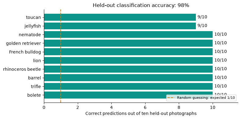
What do the mistakes look like? The next grid shows up to three mistakes first, followed by correct predictions from different categories. Each title gives the dataset label and the classifier’s prediction. Red means incorrect and green means correct. These are deliberately selected examples, not a random sample or another accuracy estimate.
test_rows = np.flatnonzero(~train_mask)  # Match test-vector order to the photograph list.
example_indices = list(np.flatnonzero(~correct)[:3])
for k in range(len(probe_classes)):
    matches = np.flatnonzero(correct & (y_test == k))
    if len(matches) and len(example_indices) < 6:
        example_indices.append(matches[0])

fig, axes = plt.subplots(2, 3, figsize=(10, 7))
for ax in axes.flat:
    ax.axis("off")
for ax, i in zip(axes.flat, example_indices):
    ax.imshow(Image.open(io.BytesIO(probe_pngs[test_rows[i]])))
    ax.set_title(f"Label: {probe_classes[y_test[i]]}\nPrediction: {probe_classes[test_predictions[i]]}",
                 color="#0d9488" if correct[i] else "#dc2626", fontsize=10)
plt.tight_layout()
plt.show()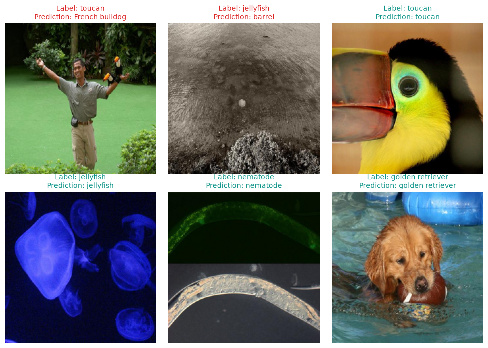
A single linear layer learned from 30 labelled examples per category and correctly classified 98 of 100 different, held-out photographs using the frozen I-JEPA features. Those features therefore contain useful information for separating these ten categories.
The two mistakes were a toucan predicted as a French bulldog and a jellyfish predicted as a barrel. In these photographs the labelled subject is much less prominent than in the correct examples, although the pictures alone cannot establish why the classifier failed.
This is a small ten-category demonstration, not a reproduction of the paper’s full ImageNet evaluation or a claim of 98% accuracy on arbitrary photographs.
I-JEPA learns image representations by predicting vectors for hidden regions. Those learned representations can then support tasks such as classification. Our four experiments connected these two uses.
| Experiment | What we did | What we learned |
|---|---|---|
| 1. Encode a photograph | Passed a 224 × 224 RGB photograph through the pretrained target encoder. | It returned 256 patch vectors, each containing 1,280 numbers. |
| 2. Predict a hidden region | Hid 16 patches from the context encoder and used the predictor to produce their vectors. | We can compare each predicted vector with the target encoder’s vector at the same position. The predictions are numbers, not reconstructed pictures. |
| 3. Change the visible context | Used ten other photographs as context, keeping the astronaut’s target vectors and hidden positions fixed. | All ten gave higher error than the astronaut’s own context. This supports the value of matching context in this particular test. |
| 4. Use the features | Trained a linear classifier on frozen target-encoder features from 300 labelled photographs. | It classified 98 of 100 held-out photographs correctly across ten categories. The features carry useful category information. |
What changed during training? In I-JEPA pretraining, backpropagation updates the context encoder and predictor. The target encoder starts as a copy of the context encoder and then follows its weights through an exponential moving average: a smooth, delayed tracking response. In our experiments, all three pretrained networks stayed fixed. Only our small classifier learned new weights.
The 98% result belongs to this small classification test, not arbitrary images or the paper’s full benchmark. We have now followed I-JEPA from its prediction task to a practical use of its learned features.
Community
Share what you’re learning, ask questions, and swap ideas.
Join the ExploringML Discord.