V-JEPA: Learning Video Representations by Feature Prediction
Follow V-JEPA ViT-L/16 from video tubelets and feature prediction to pretrained encoder features, temporal tests and a small action-classification experiment.
JEPA
Computer Vision
Deep Learning
Video
Python
Author
David Gwyer
Published
September 25, 2026
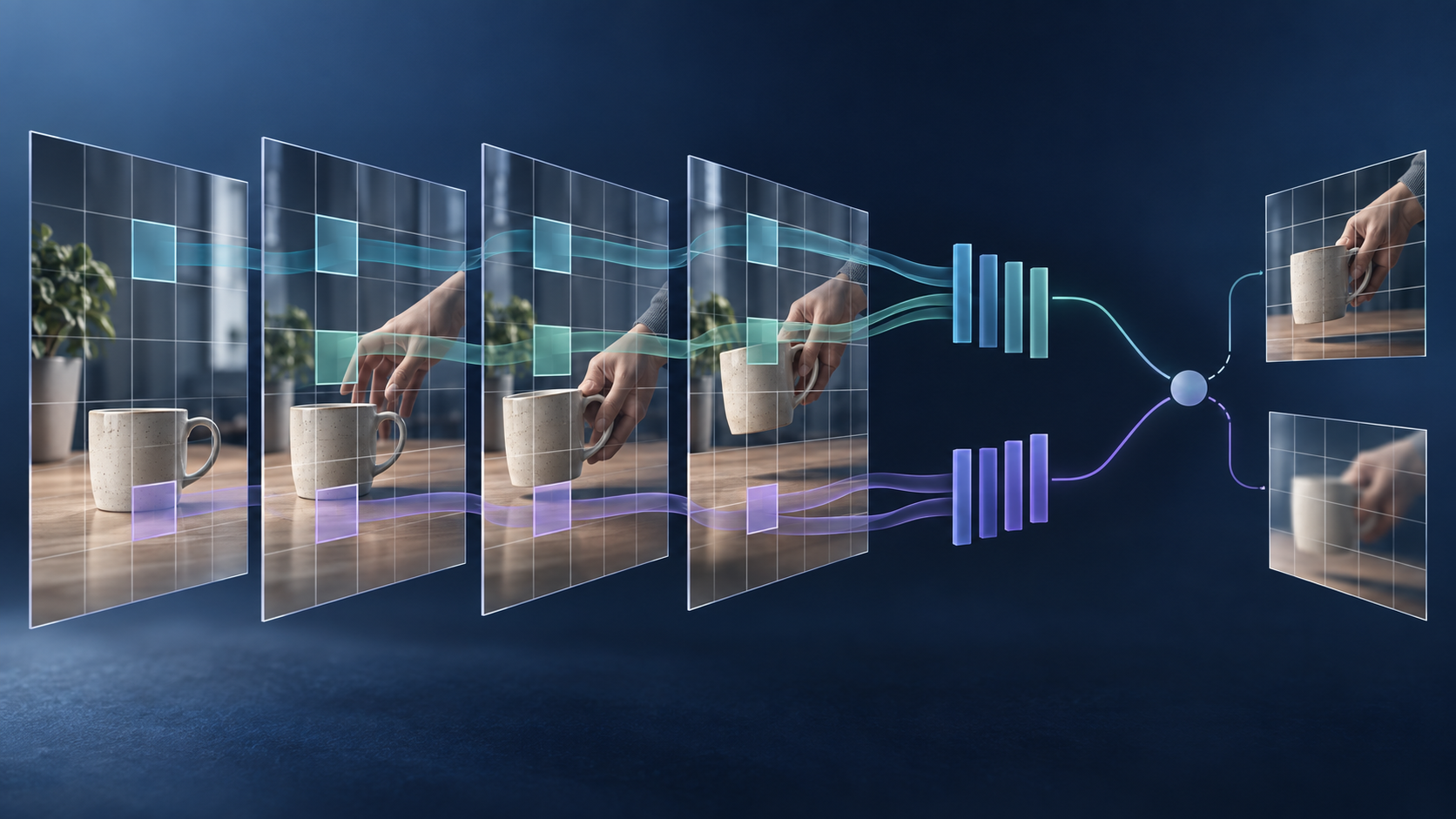
A hand lifts a cup across video frames divided into patch grids, with teal and violet feature streams feeding predicted frames.
This article follows V-JEPA from its video input to a pretrained encoder and a few small experiments. The complete notebook, including saved outputs and setup notes, is available as a downloadable ZIP, or you can read the interactive SolveIt dialogue.
JEPA stands for Joint-Embedding Predictive Architecture. It is an architecture and training approach for learning representations by predicting one part of an input from another in feature space. I-JEPA applies this idea to images, and V-JEPA extends it to video, where the model can learn from changes across frames. Both predict feature vectors rather than reconstructing pixels.
For the original I-JEPA and V-JEPA, the encoder is the main result of pretraining. It turns an image or video into features that other models can use. A "V-JEPA model" can therefore mean the pretrained encoder produced by this process, as well as the architecture used to train it.
One Pretraining Step
Take a video of a hand lifting a cup and hide some patches from the context branch. The context encoder represents the visible content. A smaller predictor uses those features to estimate vectors for the hidden positions. The target encoder sees the full clip and supplies the vectors used to check those predictions.
The two diagrams presented below follow the forward pass of one pretraining step: computing features, making predictions and measuring their error. Each prediction is compared with the target vector at the same position in space and time. The weight updates that follow this comparison complete the training step.
A tubelet is a video patch that spans consecutive frames. Here, it covers the same 16 × 16-pixel region in two sampled frames. The embedding layer turns each tubelet into a 1,024-value vector, then adds a position vector of the same size.
The resulting vector represents one token, an item in the transformer's input sequence. It carries information about the tubelet's content and its position in space and time. The context branch keeps only the visible tokens; the transformer then updates each one using information from the others.
flowchart TD
 X["Video clip<br/>16 sampled RGB frames<br/>224 × 224 pixels each"]
 subgraph C["CONTEXT ENCODER"]
 C1["Patch embedding layer<br/>Each RGB tubelet:<br/>2 frames × 16 × 16 pixels<br/>Learned projection<br/>1,024 values per tubelet<br/>1,568 vectors per clip"] --> C2["Add position vectors<br/>1,024 + 1,024 → 1,024"]
 C2 --> C3["Keep visible tokens<br/>Remove hidden tokens"]
 C3 --> C4["Transformer blocks<br/>Attention across<br/>visible tokens<br/>Final layer normalisation"]
 end
 subgraph T["TARGET ENCODER"]
 T1["Patch embedding layer<br/>Each RGB tubelet:<br/>2 frames × 16 × 16 pixels<br/>Learned projection<br/>1,024 values per tubelet<br/>1,568 vectors per clip"] --> T2["Add position vectors<br/>1,024 + 1,024 → 1,024"]
 T2 --> T3["Keep all tokens"]
 T3 --> T4["Transformer blocks<br/>Attention across<br/>all tokens<br/>Final layer normalisation"]
 end
 X ----> C1
 X ----> T1
 C4 --> V["Visible features<br/>To predictor below"]
 T4 --> F["Full-clip features<br/>To target selection below"]
 classDef online fill:#eef4fa,stroke:#7392ad,color:#243447
 classDef teacher fill:#f0f7f5,stroke:#7b9c92,color:#243447
 class C1,C2,C3,C4,V online
 class T1,T2,T3,T4,F teacher
 style C fill:#fafcfe,stroke:#a6b8c8
 style T fill:#f9fcfb,stroke:#a1b9b0
Each tubelet covers the same 16 × 16-pixel region in two sampled frames. It contains 2 × 16 × 16 × 3 = 1,536 RGB values. The patch embedding layer maps this whole block to one 1,024-value vector using a learned 3D convolution. It reads the values from both frames together; it does not first add or average the two patches. Grouping the pixels into tubelets and projecting them are performed by this layer.
A 224 × 224 frame has 14 × 14 spatial positions. Sixteen sampled frames form eight pairs, giving 8 × 14 × 14 = 1,568 tubelets and therefore 1,568 initial embedding vectors per clip. Each receives a 1,024-value position vector through elementwise addition. The context branch then removes hidden tokens before attention; the target branch retains all of them. Patch embedding layer, encoder.
Attention lets each token use information from other tokens in its input sequence. The context transformer can attend across the retained visible tubelets; the target transformer can attend across the whole clip. Each output still corresponds to one tubelet position, but now incorporates context from other positions. Final layer normalisation normalises the values within each output vector while preserving its 1,024-value width and position in the sequence.
The predictor uses the same kind of fixed sine-and-cosine position encoding as the encoder, generated at width 384. Time, row and column encodings occupy portions of one position vector; they are not three separate 384-value vectors added to a token. Position encoding implementation.
flowchart TD
 V["Visible features<br/>1,024 values per token"]
 subgraph P["PREDICTOR"]
 R["Linear projection<br/>1,024 → 384"] --> A["For each visible token<br/>Projected feature + position<br/>384 + 384 → 384"]
 H["For each hidden position<br/>Learned mask token<br/>+ position vector<br/>384 + 384 → 384"]
 A --> J["Append placeholders<br/>to visible tokens<br/>One longer sequence<br/>384 values per token"]
 H --> J
 J --> B["12 transformer blocks<br/>Use visible context<br/>to predict hidden features<br/>Final layer normalisation"]
 B --> O["Keep hidden outputs<br/>Project 384 → 1,024"]
 end
 V ----> R
 O --> Y["Predicted vectors<br/>One per hidden position"]
 F["Full-clip target features"] --> S["Normalise features<br/>Select matching<br/>hidden positions"]
 S --> Z["Target vectors<br/>1,024 values each"]
 Y --> L["L1 loss<br/>Match hidden positions"]
 Z --> L
 L -.-> U["Weight updates<br/>Backpropagation:<br/>context encoder + predictor<br/>Target: moving average"]
 style U fill:#fffaf0,stroke:#b9a587,stroke-dasharray:4 3
 classDef online fill:#eef4fa,stroke:#7392ad,color:#243447
 classDef target fill:#f0f7f5,stroke:#7b9c92,color:#243447
 classDef mask fill:#fff1df,stroke:#c27828,color:#804a16
 class R,A,J,B,O,V,Y online
 class F,S,Z target
 class H mask
 style P fill:#fafcfe,stroke:#a6b8c8
Each visible feature is projected to 384 values, then added elementwise to its own position vector. Each hidden position instead gets a learned placeholder, called a mask token, plus its own position vector. The placeholder contains no hidden image content. Both operations produce separate 384-value token vectors.
Every forward pass starts with placeholders made from the current learned mask token and each hidden position's vector. They do not carry guesses over from the previous pass.
"Append" joins the two lists of tokens. For example, 10 visible tokens and 6 hidden-position tokens produce a sequence of 16 vectors, each 384 values wide. Attention lets the placeholders use the visible features and interact with other tokens. Their outputs become predictions for the requested hidden positions. Each requested hidden position gets one predicted vector. Sixteen hidden patches would mean sixteen predictions, but the mask determines that count; it is not fixed by the model. Predictor implementation.
These diagrams use V-JEPA ViT-L/16, with encoder width 1,024. For I-JEPA ViT-H/14, that width is 1,280. Its predictor also projects to its narrower internal width before adding predictor position vectors. I-JEPA implementation.
The dashed arrow beneath the loss marks the weight updates after the forward pass. Backpropagation uses the prediction error to update both the predictor and the context encoder. The context encoder learns to produce features that help predict the hidden content, even though it produces outputs only for visible positions.
The target encoder receives no gradient update. Its weights follow an exponential moving average of the context encoder's weights, giving a gradually changing reference. This comparison and update happen on every training step. The target vectors are used for the loss and are never fed into the predictor. V-JEPA method.
In ViT-L/16, each video patch becomes a vector with 1,024 coordinates. Spatial and temporal position information is added before the encoder's transformer processes the visible tokens.
The predictor projects the encoder outputs to 384 coordinates and adds position information at that width. Hidden positions receive learned mask tokens with their own position information. Twelve transformer blocks process the visible and hidden-position tokens together. An output projection then maps the hidden-position results back to 1,024 coordinates for comparison with the target vectors. These widths count the coordinates in each vector. The number of patch positions is a separate dimension. Configuration, predictor implementation.
The smaller predictor is intended to encourage the encoder to learn representations that make prediction easier. Reduced width alone does not guarantee useful features or prevent collapse, where different inputs produce the same representation.
After pretraining, we can use the encoder to extract features for a downstream task, meaning a task we want to solve with the learned representations. For action classification, a classifier learns to map video features to action labels. The encoder can remain frozen, with its weights fixed, or be fine-tuned for that task. Ordinary feature extraction uses the encoder without the masking, predictor or target-comparison branch.
Using the pretrained encoder for action classification:
graph LR
 V["Video clip"] --> E["Pretrained encoder"] --> F["Video features"] --> C["Trained classifier"] --> A["Action label"]
 classDef model fill:#eef4fa,stroke:#7392ad,color:#243447
 class E,C model
Once the classifier has been trained, this forward pass produces a prediction for a new clip. No weight update is needed for inference.
What Changes When the Picture Moves?
A photograph shows the hand and cup at one instant. Across a video, their positions change: the hand approaches, grips the cup and lifts it. V-JEPA's input includes these changes over time, while I-JEPA receives a single image.
An image supplies patches arranged in rows and columns. A video adds a time dimension: each patch covers a fixed region across consecutive sampled frames. Those pixels become embedding vectors, which form the token sequence processed by the transformer.
The original V-JEPA method predicts hidden regions within a clip. The visible context can include information from across that clip, so this training task should not be treated as evidence of forecasting future events or planning actions.
Now that we understand the architecture, we can see what V-JEPA's representations look like in practice. We'll take a real video clip, select a few frames, and inspect the features produced by the pretrained encoder. Then we'll hide parts of the clip and examine what the model predicts for them.
Because V-JEPA is designed for video, we'll also change the temporal information and observe how its representations respond. Finally, we'll train a small action classifier on top of frozen encoder features. This won't reproduce a full benchmark, but it will give us a concrete test of what the model has learned from our examples.
The pretrained weights and GPU-intensive computation will run on Modal, and the results will be returned directly.
The Model We'll Explore
We'll use Meta's original V-JEPA ViT-L/16 with 224 × 224-pixel input frames. Its released checkpoint, vitl16.pth.tar, is listed in Meta's model zoo. It is smaller than the ViT-H variants.
The table gives its input dimensions and encoder feature width, which is the number of coordinates in each output vector.
A video patch contains the same 16 × 16-pixel region across two sampled frames. Its location stays fixed in the image while objects can move through it.
The model converts these pixels into an embedding vector. That vector occupies one position in the transformer's input sequence, where we call it a token. "Patch" describes the raw input region, "embedding" its numerical representation, and "token" its place in the sequence.
The official configuration uses sampling_rate: 4, so consecutive frames in the model's input need not be adjacent in the source video. We first sample frames, then group that sequence into pairs.
When we load the checkpoint, we'll check for the context-encoder, target-encoder and predictor weights needed for the hidden-region experiment.
Count the Video Patches
I-JEPA ViT-H/14 divides a 224 × 224 image into 14 × 14-pixel patches, giving 16 rows × 16 columns = 256 tokens. V-JEPA ViT-L/16 uses larger spatial patches, so each frame pair has 14 rows × 14 columns = 196 positions.
Sixteen sampled frames give eight non-overlapping pairs. Multiplying the grid dimensions gives the total token count as shown below. Note: The // operator performs whole-number division.
The output ((8, 14, 14), 1568) gives the grid in (time, rows, columns) order and the total of 1,568 tokens. It counts patch positions; it does not contain their learned vectors.
Next, we'll select the 16 input frames from an actual video.
Choosing the Frames
We'll use a short basketball clip from UCF101, also used in Hugging Face's video-classification guide. A player moving towards the basket gives us motion to follow across the sampled frames.
For this first inspection, we'll take 16 frames at a spacing of four source frames. We'll display them before resizing or normalising the pixels. This is lightweight video preparation in SolveIt; the encoder and GPU work will run on Modal later. OpenCV will decode the video, so the next cell installs the package we need.
The cell above downloads the clip if needed and reports its filename and file size in bytes. Here's the five-second video. Play it to see the movement, then compare it with the sampled frames below.
import subprocessfrom IPython.display import Video# Convert the AVI clip to a browser-friendly MP4 for playback.preview_path = video_path.with_suffix(".mp4")subprocess.run(["ffmpeg", "-y", "-loglevel", "error", "-i", str(video_path),"-c:v", "libx264", "-pix_fmt", "yuv420p", "-c:a", "aac","-movflags", "+faststart", str(preview_path)], check=True)Video(str(preview_path), embed=True, width=560)
cap = cv2.VideoCapture(str(video_path))ifnot cap.isOpened():raiseRuntimeError("Could not open the video")fps = cap.get(cv2.CAP_PROP_FPS)frame_count =int(cap.get(cv2.CAP_PROP_FRAME_COUNT))source_size = (int(cap.get(cv2.CAP_PROP_FRAME_WIDTH)),int(cap.get(cv2.CAP_PROP_FRAME_HEIGHT)))cap.release(){"frames": frame_count, "fps": fps, "size (width, height)": source_size}
The clip has 125 frames at 25 frames per second. We'll choose a window near the middle and keep every fourth frame. That makes neighbouring sampled frames 0.16 seconds apart.
Sixteen samples contain 15 gaps, so the first and last samples will be 2.4 seconds apart. This is our simple, repeatable sampling choice for the walkthrough; training can sample different windows.
num_frames, stride =16, 4span = (num_frames -1) * stride +1if frame_count < span:raiseValueError(f"This sampling needs at least {span} source frames")start = (frame_count - span) //2frame_indices = [start + i * stride for i inrange(num_frames)]frame_indices
Frame numbers start at zero. We'll read the selected frames in order and convert OpenCV's BGR colour order to RGB for display. Each item in sampled_frames will still be a complete 240 × 320 image, with three colour channels per pixel.
sampled_frames = []cap = cv2.VideoCapture(str(video_path))try:for index inrange(frame_indices[-1] +1): ok, frame = cap.read()ifnot ok:raiseRuntimeError(f"Could not decode frame {index}")if index in frame_indices: sampled_frames.append(cv2.cvtColor(frame, cv2.COLOR_BGR2RGB))finally: cap.release()len(sampled_frames), sampled_frames[0].shape
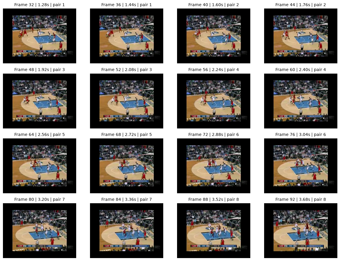
Read the grid from left to right, one row at a time. The players move towards the basket as the sequence progresses. These are the source frames, including the black borders and broadcast graphics already present in the clip.
The pair labels connect this sequence to the model's input: frames 32 and 36 form the first pair, frames 40 and 44 the second, and so on. After spatial preprocessing to 224 × 224, each pair supplies 196 tubelets. Each tubelet covers one fixed 16 × 16 region across the two frames, so a whole frame pair produces 196 tokens, not one.
We now have the 16 RGB frames. Next we'll prepare their pixel values and dimensions for the pretrained encoder.
Getting the Clip Ready for the Encoder
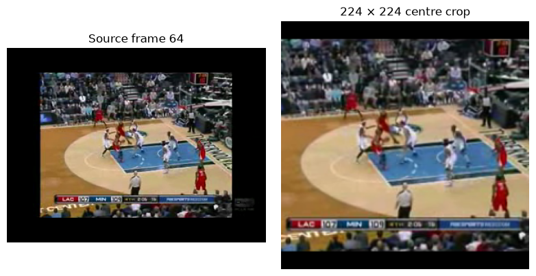
Our frames are 240 × 320 pixels. We'll resize the shorter side to 256, preserving the aspect ratio, then take the central 224 × 224 region. Every frame gets the same crop, so preprocessing does not introduce artificial camera movement.
This follows the single-view evaluation recipe in Meta's implementation. We'll write the steps out using OpenCV so we can inspect them; small interpolation differences mean this is not a bit-for-bit reproduction of that implementation.
import numpy as npdef prepare_frame(frame, short_side=256, crop_size=224): height, width = frame.shape[:2] scale = short_side /min(height, width) size = (int(width * scale), int(height * scale)) resized = cv2.resize(frame, size, interpolation=cv2.INTER_LINEAR) top = (resized.shape[0] - crop_size) //2 left = (resized.shape[1] - crop_size) //2return resized[top:top + crop_size, left:left + crop_size]cropped_frames = np.stack([prepare_frame(f) for f in sampled_frames])cropped_frames.shape
The crop removes some of the scene, so it is worth checking what remains before interpreting any model output. The array now has shape (16, 224, 224, 3): frames, height, width, RGB channels.
We'll divide the pixel values by 255, then subtract a fixed mean and divide by a fixed standard deviation for each colour channel. The constants below come from the same evaluation recipe. They are not statistics calculated from this basketball clip.
Finally, we'll put the axes in the order the encoder expects: (batch, channels, time, height, width). A batch is a group of clips processed together; ours contains just one.
permute rearranges the axes, preserving the frame order. unsqueeze(0) adds the batch axis. The result is a PyTorch tensor, a multidimensional array ready for the model. These values still represent pixels. The encoder's patch-embedding layer will turn them into tubelet embeddings.
A First Look at the Target Encoder's Learned Features
We can now pass the complete clip through V-JEPA's pretrained target encoder. The target encoder should return a 1,024-value vector at each of the clip's 1,568 tubelet positions. Attention lets each position gather information from across the clip, so these vectors describe more than isolated pixels. They are features, not action labels; recognising "basketball dunk" would still require a suitable classifier.
We'll run this target-encoder-only feature extraction on a Modal GPU and return the results. First we need the Modal Python package and an authenticated connection.
A checkpoint stores learned weights. We'll use vitl16.pth.tar from Meta's model zoo. The file contains weights for the context encoder (encoder), target encoder (target_encoder) and predictor, but this walkthrough selects onlycheckpoint["target_encoder"], following the default in the evaluation code.
During V-JEPA pretraining, the target encoder is the moving-average encoder that supplies representation targets. Here, training is over: we use that target encoder by itself as a frozen feature extractor. The context encoder and predictor remain in the checkpoint but are neither instantiated nor run in this section.
The following code describes the remote software environment. Modal caches this environment, including the downloaded checkpoint, so subsequent runs can reuse it.
Before running the clip, we'll require every target-encoder weight to match the vit_large model definition. strict=True makes loading fail if any selected target-encoder weights are missing or unexpected, instead of silently leaving part of that encoder randomly initialised.
We'll also return the checkpoint's top-level keys to verify which components the file contains for later experiments. Seeing encoder, target_encoder and predictor in that list does not mean all three are used here: the loader extracts only checkpoint["target_encoder"].
eval() selects evaluation behaviour, while inference_mode() avoids building the gradient information needed for training. We pass the complete clip directly to the frozen target encoder, without a mask. It produces one feature vector at every tubelet position, and no weights are updated.
Nothing in this call uses V-JEPA's context encoder or predictor. Those components are central to the pretraining task, where visible context is encoded and missing-region representations are predicted, but this is inference after pretraining, using only the learned target encoder to describe the clip.
The first call also builds the remote environment and downloads the checkpoint, so it will take longer than a cached run. This uses one A10G GPU on Modal for the inference call.
asyncwith vjepa_app.run.aio(): encoder_result =await encode_clip.remote.aio(clip_tensor.cpu().numpy())features = encoder_result["features"]checkpoint_keys = encoder_result["checkpoint_keys"]components = ["encoder", "target_encoder", "predictor"]missing = [key for key in components if key notin checkpoint_keys]assertnot missing, f"Missing checkpoint components: {missing}"print(f"Checkpoint contains: {', '.join(components)}\n"f"This run used: {encoder_result['encoder_weights']}\n"f"Encoded clip: {features.shape}\n"f"JEPA revision: {encoder_result['source_revision'][:8]}")
Checkpoint contains: encoder, target_encoder, predictor
This run used: target_encoder
Encoded clip: (1, 1568, 1024)
JEPA revision: 51c59d51
The returned shape is (1, 1568, 1024): one clip, 1,568 target-encoder positions and 1,024 values per position. Strict loading passed for the selected target-encoder weights.
The checkpoint also contains encoder and predictor weights, but their presence should not be confused with execution: this run loaded and called only target_encoder. No context-encoder or predictor outputs contribute to features.
We can arrange the 1,568 positions back into the familiar grid of eight frame pairs, 14 rows and 14 columns. That only changes how we index the target encoder's output. Each vector already includes information gathered from across the clip through the target encoder's attention layers.
Those are the first 12 values of one 1,024-value target-encoder vector. Row and column indices start at zero. Individual coordinates do not come with labels such as "ball" or "player", so this list alone tells us little about what the target encoder has learned. Comparing its vectors across positions or under controlled changes to the clip will be more informative.
These saved features are target-encoder representations only; they contain no separately computed context-encoder representation and no predictor output. We can save the complete features and the source-code revision here, so inspecting this result again does not require another GPU run.
We will now ask a concrete JEPA-style question: given only the tubelets outside a central region, can the pretrained model predict the learned features that the complete clip would have produced inside that region?
The 16-frame input is divided into non-overlapping tubelets. Each tubelet covers one 16 × 16 spatial area across two consecutive sampled frames. There are eight frame pairs and a 14 × 14 spatial grid in each pair, so the clip contains
[ 8 = 1{,}568 ]
tubelet positions.
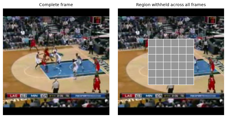
We will withhold the central 6 × 6 positions in every frame pair. That hides 36 tubelets per pair, or (8 = 288) positions across the clip. The other 1,280 positions remain visible.
Three frozen components from the pretrained checkpoint have separate roles:
The context encoder (encoder) receives only the 1,280 visible tubelets and turns them into context features.
The predictor receives those visible features, the locations of the visible and hidden tubelets, and learned mask-token placeholders. It predicts one 1,024-value feature vector for each of the 288 hidden positions.
The target encoder (target_encoder) receives the original, complete clip. Its feature vectors at those same 288 positions provide the reference targets.
We then compare each predicted vector with the target-encoder vector at the same tubelet position. This is feature prediction, not image reconstruction: the model will not generate pixels or a viewable replacement for the hidden square. No weights are updated in this experiment.
This creates a tubelet mask for the clip. In every one of the eight frame pairs, the central 6 × 6 region is marked as hidden. Flattening the mask produces indices for the 288 hidden tubelets and the remaining 1,280 visible tubelets; these tell V-JEPA what context it may see and which positions it must predict.
The grey block shows which spatial locations we chose to withhold. Remember though, the model is not given a clip with a grey square painted over it.
The patch-embedding layer first divides the input into separate, non-overlapping tubelets. We then use the position indices to keep only the 1,280 visible tubelet embeddings before the context encoder's attention layers. The 288 hidden tubelets therefore contribute no pixel information to the context encoder. Because each hidden tubelet spans two frames, "hidden patch" here means the same 16 × 16 location across one sampled frame pair.
The hidden region stays at grid rows 4–9 and columns 4–9 for all eight frame pairs. This simple fixed block makes the data flow easy to inspect, although it is not the varied random multi-block masking recipe used during V-JEPA pretraining.
For the forward pass we load all three relevant checkpoint components and keep them frozen:
encoder for the visible context;
predictor for estimating features at hidden positions;
target_encoder for producing reference features from the complete clip.
The following code constructs these models with the same video and tubelet geometry used earlier and requires every checkpoint weight to match with strict=True.
def load_prediction_models():import torchfrom src.models.vision_transformer import vit_largefrom src.models.predictor import vit_predictor checkpoint = torch.load("/opt/vitl16.pth.tar", map_location="cpu", weights_only=True) settings =dict(img_size=224, patch_size=16, num_frames=16, tubelet_size=2, uniform_power=True) models = {key: vit_large(**settings) for key in ("encoder", "target_encoder")} models["predictor"] = vit_predictor(**settings, embed_dim=1024, predictor_embed_dim=384, depth=12, num_heads=16, use_mask_tokens=True, num_mask_tokens=2)for key, model in models.items(): weights = {k.removeprefix("module.").removeprefix("backbone."): vfor k, v in checkpoint[key].items()} model.load_state_dict(weights, strict=True) model.eval().requires_grad_(False).to("cuda")return models
The predictor must know where it is being asked to make predictions, but it must not receive the hidden visual content. It gets:
the context encoder's features for the 1,280 visible positions;
the indices of those visible positions;
the indices of the 288 hidden positions; and
a learned mask-token vector as a placeholder at each hidden position.
Position information added inside the predictor distinguishes, for example, a hidden tubelet near the basket in the first frame pair from one at the same spatial location later in the clip. Attention in the predictor can then combine information from all visible context features when estimating each hidden feature.
The checkpoint contains two learned mask-token vectors because pretraining used two masking configurations. We select the first with mask_index=0; this is a fixed experimental choice, not a class label.
In this mask-token mode, the predictor does not take target-encoder features as input. Passing None as its second argument makes that separation explicit. Its output is 288 predicted vectors, each with 1,024 values. The target features enter only later, when we measure prediction error. Predictor implementation.
The target side supplies the answer against which the predictions are judged. The frozen target_encoder processes the original complete clip, including the region withheld from the context encoder. As in the training code, we layer-normalise each 1,024-value target vector and then select the same 288 tubelet positions requested from the predictor.
The comparison is therefore position-for-position and like-for-like:
predicted feature for one hidden tubelet: 1,024 values;
target-encoder feature for that same tubelet: 1,024 values.
For each position we take the absolute difference in every coordinate and average the 1,024 differences. Averaging those position errors gives the overall mean L1 feature error. This value is neither a pixel error nor a percentage accuracy.
The function also performs a separate masking sanity check. It makes a copy of the already-normalised input tensor and replaces values in the withheld pixel region with zero, while keeping the visible and hidden position lists unchanged. It then repeats the context-and-predictor pass. If hidden tubelets have truly been removed before the context encoder, changing their underlying pixel values cannot affect the predictions. Here, zero means zero in the normalised tensor; the particular replacement is unimportant because those tubelets should never be observed.
{'mean L1': 0.5021489858627319,
 'max change after replacing hidden pixels': 0.0}
The arrays have the expected shape (1, 288, 1024): one clip, 288 hidden tubelet positions, and a 1,024-value vector at each position.
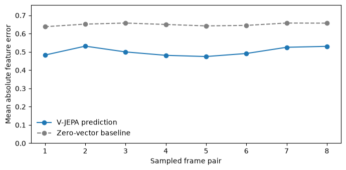
The overall mean L1 error is about 0.502. To obtain it, we compare every predicted vector with the full-clip target-encoder vector at the same hidden position, average the 1,024 absolute coordinate differences for that position, and then average over all 288 positions. Smaller values mean the predicted features are closer to the target features, but 0.502 has no direct interpretation as "50.2% wrong."
Changing the pixel values under the withheld region changed the predictions by exactly 0.0 in this run. That is an important implementation check: those hidden pixels did not leak into the context features. It does not mean the hidden region was predicted perfectly; the non-zero L1 error measures the remaining disagreement between predictions and targets.
An error number is easier to interpret with a reference. We will therefore compare the predictor with a deliberately uninformed baseline that predicts a vector of 1,024 zeros at every hidden position. Both methods are evaluated against exactly the same layer-normalised target vectors.
For every sampled frame pair, the pretrained V-JEPA predictor is closer to the complete-clip target features than the zero-vector baseline. Averaged across all hidden positions, its mean L1 error is about 0.502, compared with 0.650 for the baseline.
This supports a limited but useful conclusion: from the visible tubelets and their arrangement in space and time, the frozen context encoder and predictor recover some information about the target encoder's representation of the withheld region. The predictor is doing more than returning an uninformative zero vector.
The experiment does not show that the model reconstructed the hidden pixels, recognised the action, found the ball, or understood the scene in a human sense. The 1,024 feature coordinates do not carry individual labels, and this single clip, fixed mask, and simple baseline are only a sanity check. The remaining gap between prediction and target is feature-space disagreement.
It also does not isolate what information produced the advantage. The predictor may use spatial appearance, temporal change, player layout, camera motion, or combinations of these. A useful next experiment is to alter or remove temporal information while controlling the image content, then repeat the same position-for-position feature comparison.
This saves the hidden-region experiment locally in SolveIt as a compressed NumPy archive, so we can inspect the results later without repeating the GPU inference. Along with the predicted and target feature vectors, the file records the visible and hidden tubelet positions, per-position errors, sampled source frames, masking sanity-check result, selected mask token and JEPA source revision. Keeping this metadata with the arrays makes the result easier to interpret and reproduce.
The archive can be reopened with np.load("vjepa_hidden_region.npz"); its contents are then available by name, such as data["predictions"] and data["targets"].
What Changes When Time Runs Differently?
The previous experiment used spatial masking while leaving the clip's timeline intact. We can now hold the 16 sampled images fixed and change only their order. If V-JEPA represented a clip as an unordered collection of pictures, these changes would make no difference. Its tubelets and temporal position vectors give us reason to expect otherwise.
We'll make two altered clips. One swaps the two frames inside every tubelet pair. The other reverses the complete sequence. Both contain exactly the same normalised frames as the original, with no new pixels and none removed.
The within-pair version keeps each pair in the same temporal slot but reverses its two frames: (32, 36) becomes (36, 32). This tests whether a two-frame tubelet responds to local direction.
The fully reversed version also moves the pairs to different temporal slots. When we compare its outputs with the original, we'll reverse the eight output groups back into source-pair order. Matching positions will then refer to the same two source frames and spatial patch, although the model encountered them in the opposite temporal direction.
We'll use the same frozen target encoder and the same preprocessing as before. Each clip is encoded separately, so the GPU does not mix information between variants. The output for each one remains (1, 1568, 1024).
Cosine similarity compares the direction of two feature vectors while ignoring their overall length. A value of 1 means identical direction, 0 means no directional alignment, and negative values point in opposing directions.
We'll calculate it for matching spatial positions and source-frame pairs, then average over the 196 positions in each pair. For the fully reversed clip, this requires reversing the eight output groups before comparison.
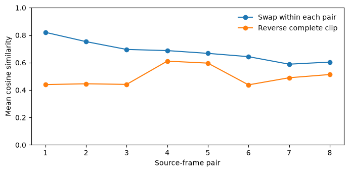
Swapping the two frames inside every tubelet pair gives a mean cosine similarity of about 0.683. The source images, pair membership and temporal slots are unchanged, so the drop from 1 shows that frame order inside a tubelet affects the encoder's features.
Reversing the complete clip lowers the aligned mean similarity to about 0.497. That change includes the reversal inside each pair, different temporal positions for the pairs, and attention across the reversed sequence. This experiment shows sensitivity to temporal order on one clip. It does not establish that the encoder recognises the action, understands cause and effect, or would respond the same way across a dataset.
The stronger response to complete reversal is consistent with a representation that uses information over time as well as appearance. It is not possible to assign that extra change to one mechanism from this comparison alone, because temporal position and cross-token attention change together.
The next section will ask a more practical question: can a small classifier use frozen V-JEPA features to separate actions without changing the encoder?
As with the earlier feature-extraction and hidden-region experiments, we save these results locally in SolveIt as a compressed NumPy archive. This avoids repeating the GPU inference when we return to the temporal-order comparison.
This archive records the target-encoder features for the original, within-pair-swapped and fully reversed clips; the corresponding source-frame orders; the position-wise cosine similarities; and the JEPA source revision used for the run. Keeping the orders and revision beside the arrays makes the comparison easier to interpret and reproduce.
It can be reopened with np.load("vjepa_temporal_order.npz"). Its contents are then available by name, including data["features"], data["pair_swap_cosine"] and data["reverse_cosine"].
Can Frozen V-JEPA Features Separate Actions?
Pretraining tells us how V-JEPA learns, but the practical question is what its encoder is useful for afterwards. We'll test that with a linear probe: freeze the released target encoder, reduce each clip to one feature vector, and train only a linear classifier to distinguish three actions.
The experiment has four stages:
choose clips from Archery, BabyCrawling, and BasketballDunk;
preprocess each clip into the same 16-frame input used above;
average the encoder's 1,568 output tokens into one 1,024-value clip representation; and
fit a three-way linear classifier on those frozen representations.
A linear probe is deliberately limited. If it separates the actions, the class information was already accessible in the pretrained features; the classifier did not teach the encoder a new representation. We use the target encoder here for consistency with the preceding feature experiments and Meta's frozen-evaluation default.
This is a small demonstration rather than a UCF101 benchmark: only 18 clips are used, from three visually distinct classes. To make the test more meaningful, we split by UCF101 recording group rather than by individual clip. Four groups per class are used for training and two different groups for testing, so near-duplicate clips from the same original recording cannot appear on both sides.
The probe reuses the Modal app, checkpoint image, and strict target-encoder loader from the earlier experiments. The only additional remote dependency is OpenCV, which decodes the UCF101 videos. The next cell adds OpenCV to that environment; the following check spells out the expected clip shape and resulting tubelet count.
The downloaded UCF101 subset contains several clips from each recording group. We keep one clip per group, then assign the first four groups in each class to training and the next two to testing. The important unit of separation is the group, not the filename: clips cut from one recording stay on only one side of the split.
def download_probe_subset():import tarfile, urllib.requestfrom pathlib import Path root = Path("/tmp/ucf101")ifnotany(root.rglob("*.avi")): root.mkdir(parents=True, exist_ok=True) archive ="/tmp/UCF101_subset.tar.gz" urllib.request.urlretrieve("https://huggingface.co/datasets/sayakpaul/ucf101-subset/resolve/main/UCF101_subset.tar.gz", archive)with tarfile.open(archive) as bundle: bundle.extractall(root, filter="data")return rootdef select_probe_clips(root):import re classes = ["Archery", "BabyCrawling", "BasketballDunk"] selected = []for label, class_name inenumerate(classes): files =sorted(p for p in root.rglob("*.avi")if p.name.startswith(f"v_{class_name}_")) by_group = {}for path in files: group =int(re.search(r"_g(\d+)_", path.name).group(1)) by_group.setdefault(group, path) groups =sorted(by_group)[:6] selected += [(by_group[g], label, "train"if i <4else"test")for i, g inenumerate(groups)]return classes, selected
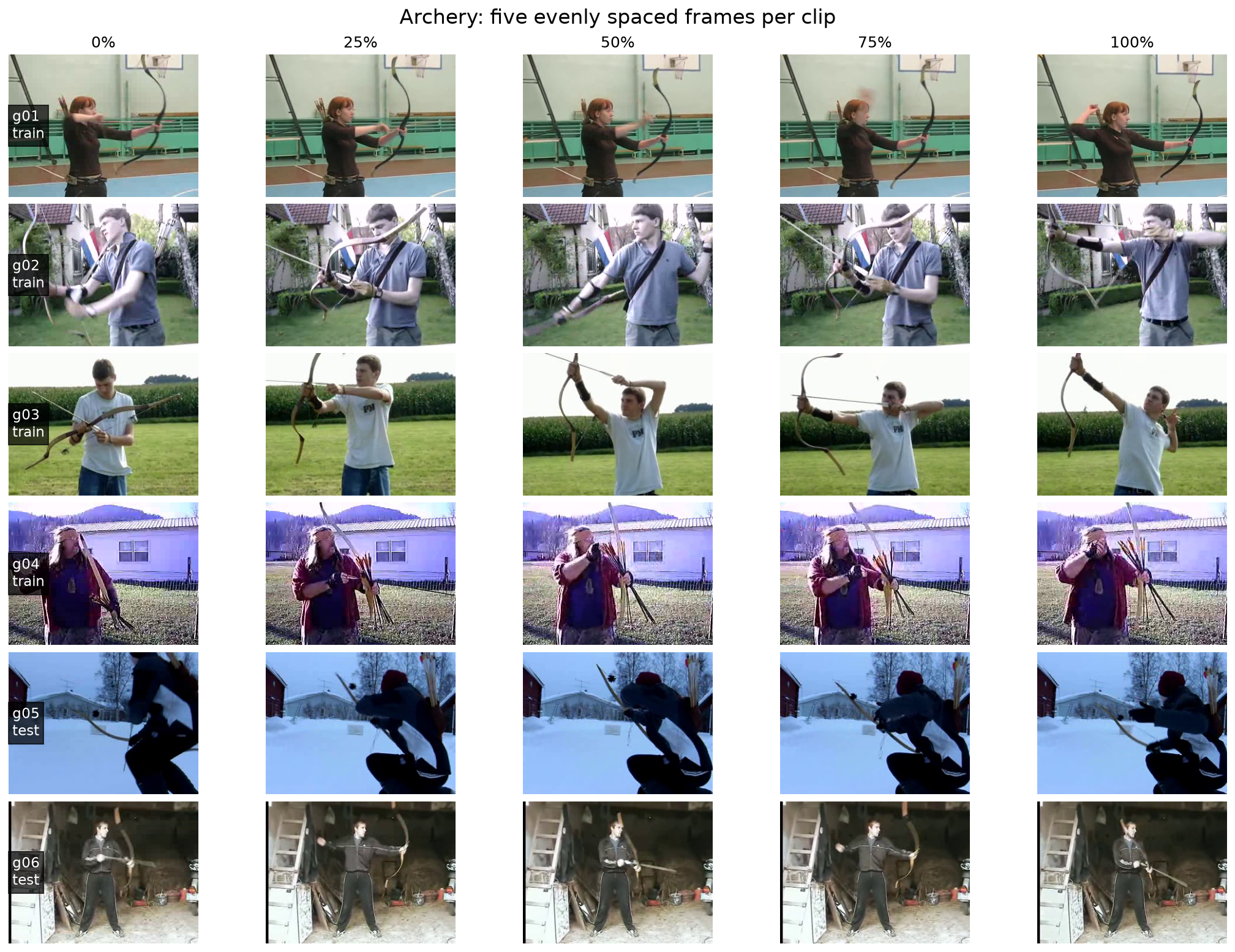
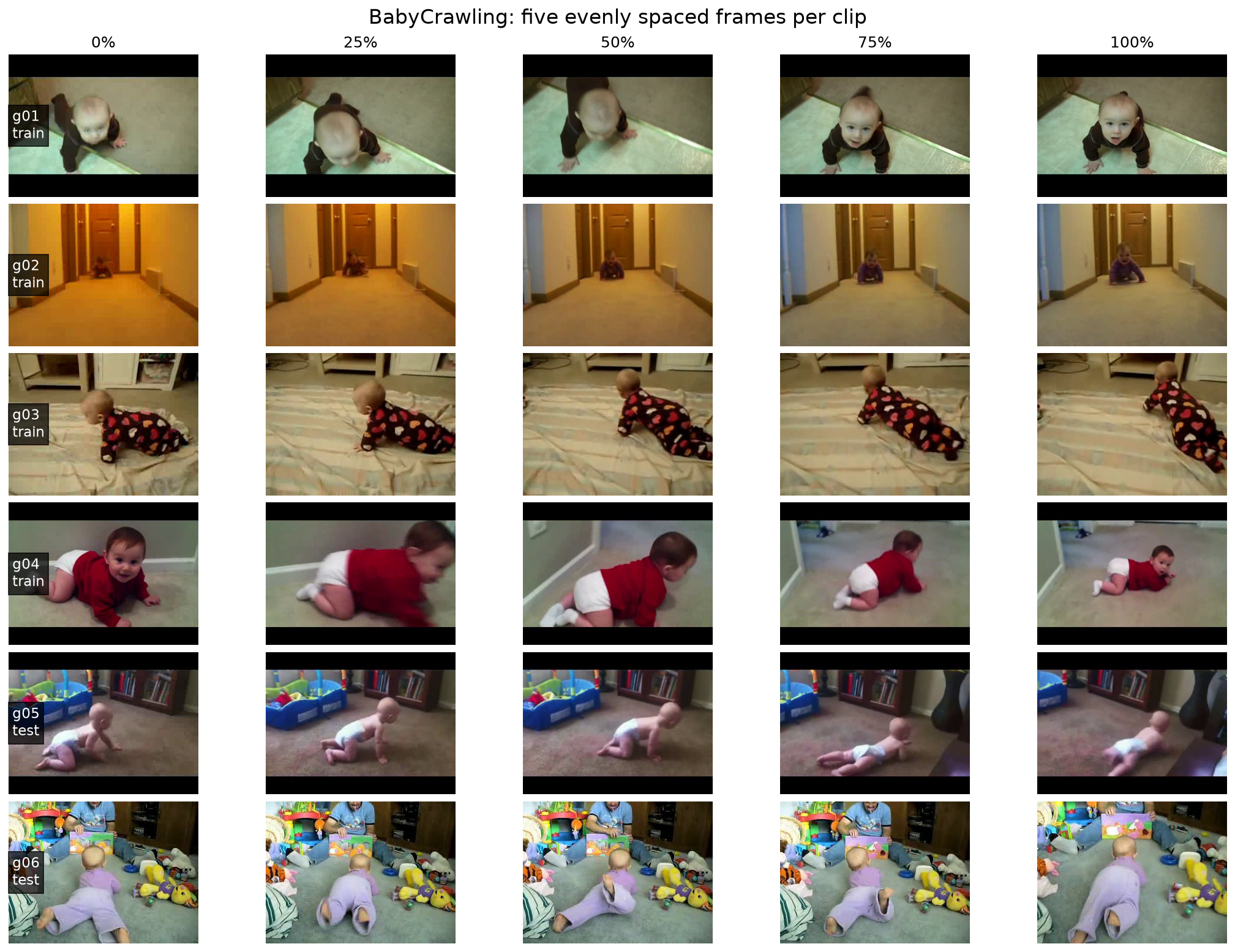
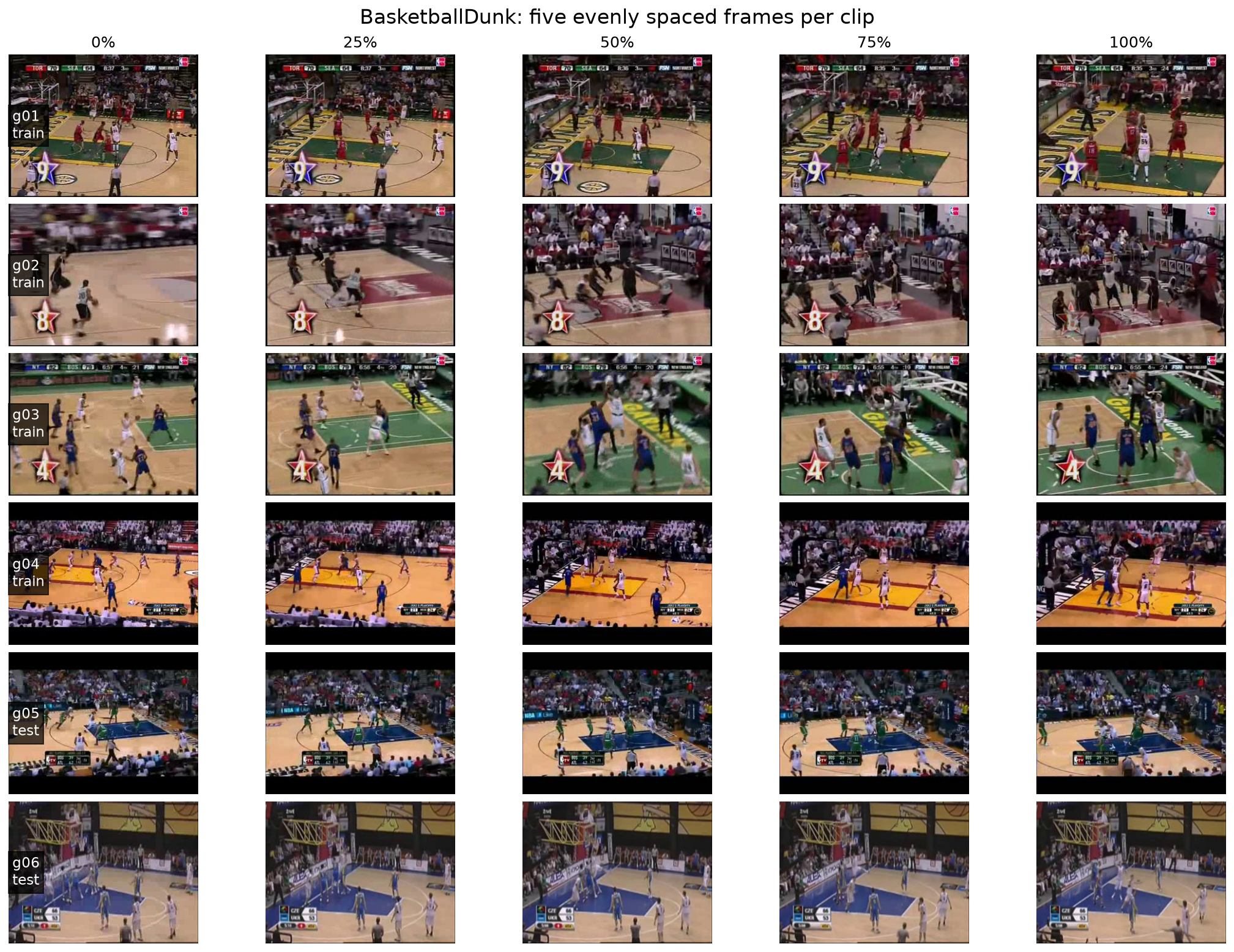
Before preprocessing the clips, we can inspect the exact sample used by the probe. Each row below is one selected recording-group clip; the five columns show evenly spaced source frames from beginning to end. The row labels identify the action and whether the clip belongs to the training or held-out split.
This is a useful visual check for near-duplicate scenes, uninformative opening or closing frames, and background cues that might make the small classification task easier than the action itself.
import cv2root = download_probe_subset()classes, selected = select_probe_clips(root)for label, class_name inenumerate(classes): rows = [(path, split) for path, y, split in selected if y == label] fig, axes = plt.subplots(len(rows), 5, figsize=(15, 11), dpi=140, layout="constrained", squeeze=False)for row, (path, split) inenumerate(rows): cap = cv2.VideoCapture(str(path)) count =int(cap.get(cv2.CAP_PROP_FRAME_COUNT)) frame_ids = np.linspace(0, max(count -1, 0), 5).round().astype(int)for col, (ax, frame_id) inenumerate(zip(axes[row], frame_ids)): cap.set(cv2.CAP_PROP_POS_FRAMES, int(frame_id)) ok, frame = cap.read()ifnot ok:raiseRuntimeError(f"Could not read {path} at frame {frame_id}") ax.imshow(cv2.cvtColor(frame, cv2.COLOR_BGR2RGB)) ax.axis("off")if row ==0: ax.set_title(f"{col *25}%", fontsize=13) cap.release() group = path.stem.split("_")[-2] axes[row, 0].text(0.02, 0.5, f"{group}\n{split}", transform=axes[row, 0].transAxes, va="center", ha="left", color="white", fontsize=12, bbox={"facecolor": "black", "alpha": 0.7, "pad": 3}) fig.suptitle(f"{class_name}: five evenly spaced frames per clip", fontsize=17) plt.show()
Turning Each Video into One Model Input
The source clips vary in length, so we choose 16 evenly spaced frames from the beginning to the end of each clip. Each frame then follows the same resize, centre-crop and channel-normalisation recipe used earlier.
This sampling choice is intentionally simple and deterministic. It gives every video the required shape, but it is not the multi-view evaluation protocol used for a full benchmark.
For each selected video, the target encoder produces 1,568 vectors. We average them across space and time to obtain one 1,024-value vector for the complete clip. This pooling discards the location of individual tubelets, but leaves a compact representation suitable for a small classifier.
The encoder stays in evaluation mode and no gradients are computed. The action labels are collected alongside the features, but they are never supplied to V-JEPA.
With the selection and preprocessing functions in place, we can run feature extraction once on the GPU. The returned arrays contain the pooled features, labels, split assignments and filenames needed for the local probe; the classifier itself will run in SolveIt rather than on the GPU.
The extractor returns 18 frozen clip vectors, each 1,024 values wide. For every class, four UCF101 recording groups supply the training examples and two different groups supply the test examples. That gives us 12 training clips and 6 held-out clips, with no recording group shared across the split.
The classifier is deliberately small. We normalise every clip vector to unit length, append a constant bias feature, and fit a regularised linear map from the 1,024 encoder features to three class scores. The highest score becomes the predicted action.
There are only 12 training examples but more than 1,000 feature coordinates, so regularisation matters: without it, many solutions could memorise the training set. The expression below is ridge regression written in its dual form, which solves a 12 × 12 system instead of a 1,025 × 1,025 one. Only these classifier weights learn from the labels, while V-JEPA remains frozen.
The feature matrix first converts to 64-bit floating point for a stable linear solve. Each 1,024-value clip vector is divided by its length, so the classifier compares the direction of the representation rather than allowing vectors with larger magnitudes to dominate. Appending a constant value of one gives the linear classifier a bias term.
The training labels are converted to one-hot target vectors: for example, an Archery clip has target [1, 0, 0]. Ridge regression then learns a regularised linear mapping from the frozen V-JEPA representations to three class scores. The regularisation strength is 0.1; it discourages excessively large classifier weights in this setting with many more feature coordinates than training examples.
For each clip, argmax selects the class with the highest score. Both reported accuracies are 1.0, meaning that the classifier correctly labels all 12 training clips and all 6 held-out clips. The (expected, predicted) pairs confirm that every held-out numeric label matches its prediction: class 0 is Archery, 1 is BabyCrawling and 2 is BasketballDunk.
Perfect training accuracy is not surprising with so few examples. The held-out result is more informative because its clips come from different recording groups, but six test clips are far too few to estimate performance on UCF101 generally.
The printed rows translate the numeric predictions back into class names. Each row shows the held-out filename, its expected action and the classifier's prediction. All six predictions are correct: two Archery clips, two BabyCrawling clips and two BasketballDunk clips.
The resulting held-out accuracy is therefore \(6/6 = 100\%\), compared with a 33% chance level for three balanced classes. This demonstrates that these three actions are linearly separable in this small sample of frozen V-JEPA features. It does not establish 100% accuracy on new videos or on the full 101-class dataset; the actions are visually distinct and the test set is intentionally small.
Finally, vjepa_linear_probe.npz saves the frozen features, labels, split assignments, filenames, learned classifier weights and class names. This lets us inspect or reuse the probe without downloading the videos and running the encoder again.
Reading the Held-Out Result
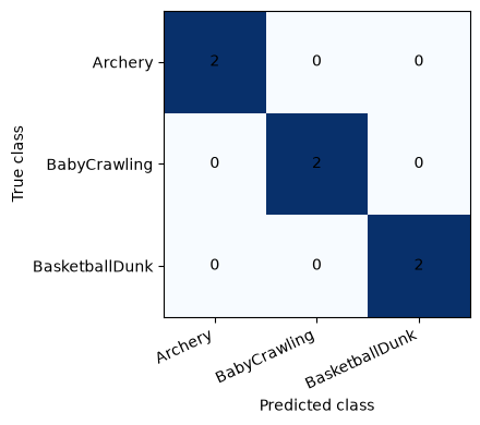
All six held-out predictions are correct. The confusion matrix below shows their distribution across the three classes.
Rows are the true classes, columns are the predicted classes, and each cell counts clips. A perfect result places all six clips on the diagonal.
The linear probe correctly classifies all six held-out clips, compared with a random 33% chance level for three classes. Its input is only the frozen 1,024-value clip vector. The V-JEPA encoder is never updated, so the result gives us direct evidence that its representation already separates these actions in this small sample.
The sample is far too small for a performance claim. Archery, baby crawling and basketball dunking are visually distinct, and six test clips cannot represent the variation in UCF101. The useful point is narrower: a shallow supervised head can read action information from features learned without action labels.
The confusion matrix is completely diagonal, matching the six printed predictions. More data and more classes would be needed to test how robust this separation is, but the experiment answers our immediate question: a simple linear classifier can distinguish these three actions from frozen V-JEPA features in this small held-out sample. The encoder itself was not retrained.
Summary
We began with raw video: 16 sampled frames from a basketball clip. V-JEPA divided them into 1,568 space-time tubelets and represented each one with a vector of 1,024 learned features. Unlike a pixel-reconstruction model, V-JEPA was trained to predict these representations for hidden parts of a video from the parts it could see.
Our experiments examined that idea from three angles. First, the pretrained predictor estimated the target encoder's features for a withheld central region more accurately than a zero-vector baseline. Changing the hidden pixels had no effect on those predictions, confirming that their contents had not leaked into the visible context.
Next, we changed the order of the same 16 frames. Swapping frames within each tubelet pair changed the encoder's features, and reversing the complete clip changed them more strongly. On this example, V-JEPA's representation therefore depended on temporal order rather than treating the video as an unordered collection of images.
Finally, we froze the encoder and trained only a simple linear classifier on its clip-level features. It correctly separated archery, baby crawling and basketball dunk in a small test set drawn from held-out recording groups. This does not constitute a UCF101 benchmark, but it shows that useful action information was already accessible in the pretrained representation.
Together, these results illustrate the main idea behind V-JEPA: learning useful video representations by predicting in feature space rather than reconstructing pixels. The experiments are deliberately small: one mask, one temporal-order example and three action classes, but they make the model's data flow and capabilities concrete.