import numpy as np
import matplotlib.pyplot as plt
import pandas as pd

# One global random generator keeps a top-to-bottom rerun deterministic.
rng = np.random.default_rng(42)
pile_A = rng.normal(0, 1, 50)
pile_B = rng.normal(3, 1, 50)While reading the VISReg paper I came across the sliced-Wasserstein distance (SWD) which is one of the central topics. I’m unfamiliar with this method so I wanted to explore it in-depth in an attempt to understand it fully.
The basic idea of SWD is to compare point clouds through their shadows. Instead of matching two high-dimensional clouds directly, we project them onto many 1D lines, compare those simpler 1D views, and average the results.
We’ll tackle this step-by-step from first principles. We start with dots on a line, where Wasserstein matching is easy to see, then move to 2D clouds, random projections, and finally to the way VISReg uses SWD to regularize neural-network embeddings.
Throughout this post I mostly report squared Wasserstein-style values, written \(W_2^2\) or \(SW_2^2\), because the code averages squared differences directly. So when you see a numeric “distance” in the examples, read it as a squared estimate unless stated otherwise.
The VISReg shape term we are trying to understand has roughly this form:
\[ \mathcal L_{\mathrm{shape}} = \frac{1}{K}\sum_{k=1}^{K} \mathrm{mean}\left( \left( \mathrm{sort}(\tilde Z w_k)-q_{\mathcal N} \right)^2 \right) \]
At first glance this may look a little intimitdating, but the whole post is about unpacking this equation:
- \(w_k\): choose a random direction
- \(\tilde Z w_k\): project the embedding cloud onto that direction
- \(\mathrm{sort}(\cdot)\): sort the 1D shadow values
- \(q_{\mathcal N}\): compare against Gaussian reference quantiles
- squared difference + mean: measure how different that 1D shadow is
- average over \(K\) directions: combine many shadow views
Below is an overview of the progression of topics covered in this post.
Specifically, we’ll: 1. Start with Wasserstein matching on a 1D line. 2. See why sorting and matching by rank makes the 1D case simple. 3. Move from 1D piles to 2D point clouds. 4. Project clouds into 1D shadows, including the dot-product calculation behind each projection, and compare those shadows. 5. Average many projections to get a squared sliced-Wasserstein estimate. 6. Use toy examples to show what squared SWD estimates can detect: collapse, anisotropy, and subtler shape differences. 7. Connect the idea back to VISReg-style embedding regularization.
Comparing two piles of dots
Let’s start with a simple 1D example: two small piles of normally distributed dots sitting on a number line.
Pile A is centred near 0, while Pile B is centred near 3. The two piles have about the same spread, so the main difference is that one pile has been shifted to the right.
plt.figure(figsize=(8, 1.8))
plt.scatter(pile_A, np.zeros_like(pile_A), alpha=0.7, label="Pile A: centred near 0")
plt.scatter(pile_B, np.ones_like(pile_B), alpha=0.7, label="Pile B: centred near 3")
plt.yticks([0, 1], ["Pile A", "Pile B"])
plt.xlabel("position on the number line")
plt.ylabel("display row")
plt.title("Two piles of dots on a line")
plt.legend(loc="upper left")
plt.grid(axis="x", alpha=0.3);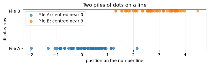
In the plot above, the vertical position does not mean anything mathematically. It is just there so we can see the two piles separately: one row for Pile A, one row for Pile B.
pd.DataFrame({
    "pile": ["Pile A", "Pile B"],
    "mean position": [pile_A.mean(), pile_B.mean()],
    "spread (std)": [pile_A.std(), pile_B.std()],
}).round(2)| pile | mean position | spread (std) | |
|---|---|---|---|
| 0 | Pile A | 0.09 | 0.76 |
| 1 | Pile B | 2.81 | 0.76 |
The table summarizes the two dot piles numerically. Their average positions are about 0.09 and 2.81, so Pile B is roughly 2.7 units to the right of Pile A. Their spreads are almost identical though, which matches the plot: the piles have similar widths, but different centres.
Matching dots by rank
Now suppose we want to compare the two piles more carefully than just looking at their averages (mean), and spread (standard deviation).
In one dimension, there’s a simple and surprisingly powerful trick: sort both piles by their positions on the number line, from left to right, then match dots with the same rank. The leftmost dot in Pile A is matched to the leftmost dot in Pile B. The second-leftmost dot is matched to the second-leftmost dot. The median-ish dot is matched to the median-ish dot. And so on.
For this example we square the distance between each pair of corresponding dots, then take the average. This gives a squared 2-Wasserstein quantity, written \(W_2^2\). In code below I call it w2_1d_sq to make the squared notation explicit.
A_sorted = np.sort(pile_A)
B_sorted = np.sort(pile_B)
movement = B_sorted - A_sorted
w2_1d_sq = np.mean(movement**2)
w2_1d_sqnp.float64(7.401410984621683)Here w2_1d_sq = 7.40, meaning the average squared movement across all 50 matched pairs is about 7.40. This is a \(W_2^2\)-style value: larger means the two 1D piles are more different, but it has squared units rather than the original position units.
The grey lines in the plot below show how each pair of points are matched. A short line means that corresponding dots are closer. A long line means that part of the pile is quite different.
plt.figure(figsize=(8, 2.4))
for a, b in zip(A_sorted, B_sorted):
    plt.plot([a, b], [0, 1], color="gray", alpha=0.25)
plt.scatter(A_sorted, np.zeros_like(A_sorted), label="Pile A sorted", zorder=3)
plt.scatter(B_sorted, np.ones_like(B_sorted), label="Pile B sorted", zorder=3)
plt.yticks([0, 1], ["Pile A", "Pile B"])
plt.xlabel("position on the number line")
plt.title(f"Matching by rank: $W_2^2$ = average squared movement = {w2_1d_sq:.2f}")
plt.legend(loc="upper left")
plt.grid(axis="x", alpha=0.3);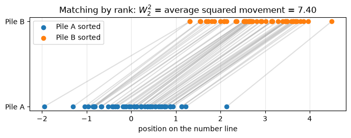
The plot matches Pile A and Pile B by rank: leftmost with leftmost, middle with middle, rightmost with rightmost.
idx = np.array([0, 12, 25, 37, 49])
pd.DataFrame({
    "rank": idx + 1,
    "A position": A_sorted[idx],
    "B position": B_sorted[idx],
    "movement B-A": movement[idx],
    "squared movement": movement[idx]**2,
}).round(2)| rank | A position | B position | movement B-A | squared movement | |
|---|---|---|---|---|---|
| 0 | 1 | -1.95 | 1.31 | 3.26 | 10.65 |
| 1 | 13 | -0.43 | 2.34 | 2.77 | 7.65 |
| 2 | 26 | 0.22 | 2.72 | 2.51 | 6.28 |
| 3 | 38 | 0.65 | 3.48 | 2.83 | 8.01 |
| 4 | 50 | 2.14 | 4.49 | 2.35 | 5.54 |
The table shows a few of those matched ranks. For each one, we record where the A dot starts, where the B dot sits, and how far apart they are.
What did rank matching measure?
This rank-matching step is the key reason 1D Wasserstein calculations are so convenient. Once the points are on a line, we do not need to solve a complicated matching problem. We sort, match by rank, and average the squared movement.
From piles of dots on a line to clouds on a plane
The 1D example was friendly because the dots had a natural order. Once both piles were sorted, we could match first with first, second with second, and so on.
Now let’s make the picture a little more realistic. Instead of dots on a number line, imagine two clouds of dots floating on a flat 2D map.
cloud_A = rng.normal([0, 0], [0.8, 0.5], size=(80, 2))
cloud_B = rng.normal([2.5, 1.2], [0.8, 0.5], size=(80, 2))
In the plot below we can see that the clouds are different: Cloud B sits up and to the right of Cloud A. But the matching trick is no longer obvious. In 2D there is no single “smallest” dot, no single “middle” dot, and no simple sorted list that tells us which points should be paired. Imagine this getting even more complicated in higher dimensions.
That is the problem sliced-Wasserstein Distance works around: rather than comparing the full 2D clouds directly, it looks at many simpler 1D views of them.
plt.figure(figsize=(5, 4))
plt.scatter(cloud_A[:,0], cloud_A[:,1], alpha=0.7, label="Cloud A")
plt.scatter(cloud_B[:,0], cloud_B[:,1], alpha=0.7, label="Cloud B")
plt.axis("equal")
plt.xlabel("x position")
plt.ylabel("y position")
plt.title("Two clouds of dots in 2D")
plt.legend()
plt.grid(alpha=0.3);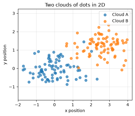
Slicing: shine a torch and compare shadows
The slicing trick is to choose a direction and project the cloud points onto the line pointing in that direction.
In 2D, the direction is a vector on the plane. In a neural-network embedding space, it might be a vector with hundreds or thousands of dimensions. The direction vector always has the same number of dimensions as the points being projected: 2 numbers for 2D points, 1024 numbers for 1024D embeddings. Either way, the idea is the same: each point is projected onto the chosen direction, turning a high-dimensional point into a single number.
Now let’s turn that idea into code for a single projection direction to start with.
We choose an angle, convert it into a unit direction vector, then project both 2D clouds onto that direction using a dot product. After projection, each cloud has become a 1D pile of shadow values. Just like before, we can then sort the two 1D piles, match by rank, square the differences, and average them.
This gives a single squared Wasserstein-style slice score. It is not the full sliced-Wasserstein estimate yet. For that, we repeat this over many directions and average the squared slice scores.
theta = np.deg2rad(25)
direction = np.array([np.cos(theta), np.sin(theta)])
shadow_A = cloud_A @ direction
shadow_B = cloud_B @ direction
slice_distance = np.mean((np.sort(shadow_A) - np.sort(shadow_B))**2)
slice_distancenp.float64(8.29801132933886)Projection asks a simple question: “how far along this direction does this point sit?”
In code, that is just a dot product:
shadow_A = cloud_A @ directionAfter this step, every 2D point has become one 1D shadow position. Once both clouds have been turned into 1D shadows, we can use the same rank-matching idea from the earlier example.
The black line in the plot below shows one such direction. It is not a physical cut through the data, just the axis we use for the projection.
fig, axes = plt.subplots(1, 2, figsize=(11, 4.2))

ax = axes[0]
ax.scatter(cloud_A[:,0], cloud_A[:,1], alpha=0.25, label="Cloud A")
ax.scatter(cloud_B[:,0], cloud_B[:,1], alpha=0.25, label="Cloud B")
axis_t = np.linspace(-2.5, 4.5, 2)
axis_pts = axis_t[:, None] * direction
ax.plot(axis_pts[:,0], axis_pts[:,1], color="black", lw=3, label="shadow axis")

example_points = np.vstack([cloud_A[[5, 20, 45]], cloud_B[[10, 30, 55]]])
example_colours = ["tab:blue"]*3 + ["tab:orange"]*3
for p, c in zip(example_points, example_colours):
    shadow = (p @ direction) * direction
    ax.plot([p[0], shadow[0]], [p[1], shadow[1]], color=c, alpha=0.8, linestyle="--")
    ax.scatter(*p, color=c, s=70, edgecolor="black", zorder=3)
    ax.scatter(*shadow, color=c, s=90, marker="x", zorder=4)
ax.set_aspect("equal")
ax.set_title("2D dots casting shadows")
ax.set_xlabel("x position")
ax.set_ylabel("y position")
ax.legend()
ax.grid(alpha=0.3)

axes[1].hist(shadow_A, bins=15, alpha=0.6, label="A shadows")
axes[1].hist(shadow_B, bins=15, alpha=0.6, label="B shadows")
axes[1].set_title(f"The 1D shadows: squared score = {slice_distance:.2f}")
axes[1].set_xlabel("position along shadow axis")
axes[1].legend();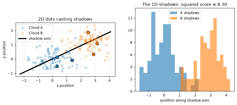
On the left in the plot above, the original 2D clouds are shown together with the chosen projection direction. A few sample points have dashed lines dropping them onto that direction, and the X markers show where their shadows land.
The right plot is a histogram visualization of the 1D shadow samples. SWD compares the sorted shadow samples directly, not the histogram bars.
pd.DataFrame({
    "object": ["Cloud A shadow", "Cloud B shadow"],
    "mean shadow position": [shadow_A.mean(), shadow_B.mean()],
    "shadow spread": [shadow_A.std(), shadow_B.std()],
}).round(2)| object | mean shadow position | shadow spread | |
|---|---|---|---|
| 0 | Cloud A shadow | -0.04 | 0.81 |
| 1 | Cloud B shadow | 2.84 | 0.75 |
The table summarizes the two projected shadow piles. Along this particular projection direction, Cloud A has mean shadow position about -0.04, while Cloud B has mean shadow position about 2.84. So in this 1D view, Cloud B’s shadow is shifted roughly 2.9 units further along the projection axis than Cloud A’s shadow. Their shadow spreads are similar, which means this slice mostly detects a location shift rather than a big change in spread.
What does one slice number mean?
A single squared slice score measures how different the two clouds look from one viewing angle.
If the projected shadows overlap closely, the squared slice score is small. If the shadows are far apart, the squared slice score is large. In the example above, the clouds are well separated along this direction, so this slice gives a fairly large squared score of 8.30.
We can calculate the same squared slice score for other arbitrary directions too, say [0, 25, 60, 90, 130].
angles = [0, 25, 60, 90, 130]
rows = []
for deg in angles:
    v = np.array([np.cos(np.deg2rad(deg)), np.sin(np.deg2rad(deg))])
    a, b = cloud_A @ v, cloud_B @ v
    rows.append({"angle degrees": deg, "squared slice score": np.mean((np.sort(a) - np.sort(b))**2)})

pd.DataFrame(rows).round(2)| angle degrees | squared slice score | |
|---|---|---|
| 0 | 0 | 6.76 |
| 1 | 25 | 8.30 |
| 2 | 60 | 5.65 |
| 3 | 90 | 1.56 |
| 4 | 130 | 0.52 |
The table shows why one slice is not enough. Some directions make the clouds look very different, while other directions make them look much closer.
Sliced-Wasserstein distance handles this by repeating the same 1D comparison across many random directions, then averaging the squared scores. Each direction gives a partial view of the cloud geometry. Averaging many of them gives a more balanced \(SW_2^2\) style estimate of how different the full clouds are.
How does the projection calculation work?
We touched on this briefly above, but let’s take a closer look at the projection calculation to make sure we have a good intuition for it. The operation is just a dot product, but it may be clearer to think of it as a temporary change of coordinates.
Suppose we choose a slice direction \(w\). We treat this direction as a new x-axis. For each point \(x\), the dot product
\[ x \cdot w \]
tells us the coordinate of \(x\) along that new x-axis.
The slice direction \(w\) is always a unit vector, meaning it has length 1. This matters because then \(x \cdot w\) is measured in the original units of the data. If \(w\) had length 2, every projected coordinate would be doubled; if it had length 0.5, every projected coordinate would be halved. Normalising \(w\) makes different slice directions comparable.
For example, if \(x=(3,2)\) and the slice direction is the horizontal unit vector \(w=(1,0)\), then
\[ (3,2)\cdot(1,0)=3. \]
So the new x-coordinate is just the usual x-coordinate.
If instead the slice direction is the 45° diagonal
\[ w=\left(\frac{1}{\sqrt2},\frac{1}{\sqrt2}\right), \]
then
\[ (3,2)\cdot w = \frac{3}{\sqrt2}+\frac{2}{\sqrt2} = \frac{5}{\sqrt2}\approx 3.54. \]
So in this rotated coordinate system, the point has coordinate about 3.54 along the diagonal axis.
In 2D, we could also compute the point’s coordinate along the perpendicular direction. If \(u\) is perpendicular to \(w\), then \(x\cdot u\) would give the new y-coordinate. But for sliced-Wasserstein distance, we deliberately ignore that perpendicular coordinate. We only keep the coordinate along the slice direction.
So each 2D point becomes one number:
\[ x \longmapsto x\cdot w. \]
For a whole cloud, the same calculation is done once per point. In code, cloud_A @ direction means: take the dot product of every point in cloud_A with the chosen unit slice direction. A 2D cloud with shape (n_points, 2) becomes a 1D array with shape (n_points,).
Higher dimensions work the same way. A 1024-dimensional embedding can be dotted with a 1024-dimensional unit direction vector. The result is still one number: the coordinate of that embedding along the chosen slice direction.
Sliced-Wasserstein distance repeats this for many random unit directions. Each direction gives one 1D view of the cloud, and those 1D views can be compared by sorting and matching by rank.
The plot below shows this change-of-axis idea visually. The coloured points are the original 2D points, and the black line is the chosen slice direction \(w\), which we can think of as a new x-axis.
For each point \(x\), the orange marker shows the location along that new axis corresponding to the dot product \(x\cdot w\). The dotted segment shows the part of the point that is perpendicular to the slice direction. Sliced-Wasserstein keeps the \(x\cdot w\) coordinate and ignores the perpendicular coordinate.
w = np.array([1., 0.35])
w = w / np.linalg.norm(w)
u = np.array([-w[1], w[0]])

P = np.array([
    [1.2, 2.8],
    [3.2, 1.8],
    [2.2, -1.2],
])

coords_w = P @ w
proj = coords_w[:, None] * w

plt.figure(figsize=(7, 6))

t = np.linspace(-1, 4.5, 100)
plt.plot(t*w[0], t*w[1], "k-", lw=2, label="new x-axis direction w")
plt.plot(t*u[0], t*u[1], "k--", lw=1.5, label="new y-axis direction u")

colors = ["tab:blue", "tab:green", "tab:purple"]
labels = ["A", "B", "C"]

for p, c in zip(P, colors):
    plt.plot([0, p[0]], [0, p[1]], color=c, alpha=0.25, lw=2, zorder=1)

for p, q, c, lab, cw in zip(P, proj, colors, labels, coords_w):
    plt.scatter(*p, s=90, color=c)
    plt.scatter(*q, s=90, color="tab:orange", edgecolor="black")
    plt.plot([p[0], q[0]], [p[1], q[1]], ":", color=c, lw=2)
    plt.text(p[0]+0.08, p[1]+0.08, f"{lab} original")
    plt.text(q[0]+0.08, q[1]-0.18, rf"{lab}: $x\cdot w={cw:.2f}$")

plt.axis("equal")
plt.grid(alpha=0.3)
plt.legend()
plt.title("Dot product gives each point's coordinate along the new x-axis");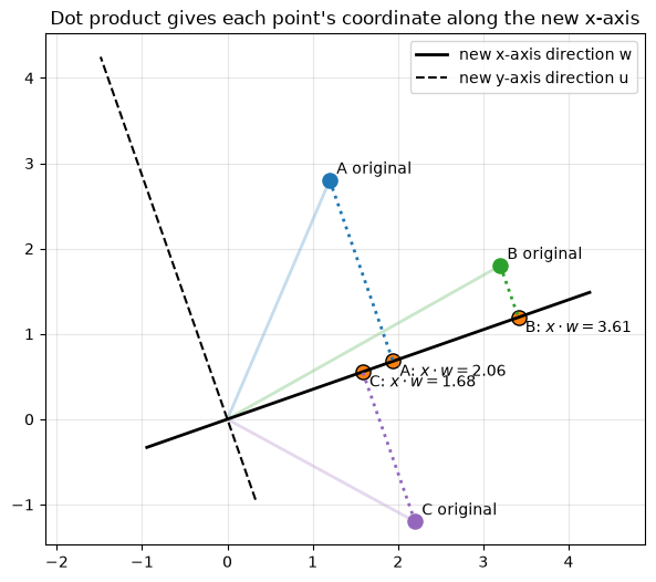
What happens in practice?
In the real paper setting, the “cloud” is a batch of neural-network embeddings, not 2D toy dots. Each image becomes one embedding vector. A batch of images becomes a high-dimensional cloud. The regularizer asks: does this ‘cloud’ have a Gaussian-like shape, or is it collapsed/squashed/weird?
In LeJEPA/SIGReg, the embeddings are pushed toward an isotropic Gaussian target: roughly (N(0, I)). In VISReg, scale and shape are separated: a variance term controls the size/spread, while the sliced-Wasserstein term compares a normalized centred embedding cloud to a Gaussian-shaped target.
So the Gaussian is like a “reference cloud”: centred, evenly spread, and not collapsed.
Many slices: one angle can fool you
A single slice is only one 1D view of the 2D clouds. Some directions show the difference clearly: the projected shadows land in different parts of the line. Other directions can hide the difference: the projected shadows overlap, even though the original 2D clouds are still separated. This is illustrated in the plot below.
def project_and_distance(cloud_A, cloud_B, deg):
    v = np.array([np.cos(np.deg2rad(deg)), np.sin(np.deg2rad(deg))])
    a, b = cloud_A @ v, cloud_B @ v
    dist = np.mean((np.sort(a) - np.sort(b))**2)
    return v, a, b, dist

deg_clear = 25
deg_hidden = 115   # almost perpendicular to 25 degrees

v_clear, A_clear, B_clear, d_clear = project_and_distance(cloud_A, cloud_B, deg_clear)
v_hidden, A_hidden, B_hidden, d_hidden = project_and_distance(cloud_A, cloud_B, deg_hidden)

fig, axes = plt.subplots(1, 3, figsize=(14, 4))

# Left: original 2D clouds with both projection directions
ax = axes[0]
ax.scatter(cloud_A[:, 0], cloud_A[:, 1], alpha=0.45, label="Cloud A")
ax.scatter(cloud_B[:, 0], cloud_B[:, 1], alpha=0.45, label="Cloud B")

pts = np.vstack([cloud_A, cloud_B])
pad = 0.5
xmin, ymin = pts.min(axis=0) - pad
xmax, ymax = pts.max(axis=0) + pad
axis_len = np.linalg.norm([xmax - xmin, ymax - ymin])
t = np.linspace(-axis_len, axis_len, 2)

for v, colour, label, offset in [
    (v_clear, "black", f"{deg_clear}° direction", np.array([0.0, 0.0])),
    (v_hidden, "purple", f"{deg_hidden}° direction", np.array([0.8, 0.0])),
]:
    axis_pts = t[:, None] * v + offset
    ax.plot(axis_pts[:, 0], axis_pts[:, 1], color=colour, lw=3, label=label)

ax.set_xlim(xmin, xmax)
ax.set_ylim(ymin, ymax)
ax.set_aspect("equal")
ax.set_title("Two possible 1D views")
ax.set_xlabel("x position")
ax.set_ylabel("y position")
ax.legend()
ax.grid(alpha=0.3)

# Middle/right: shadows for each direction
for ax, A_shadow, B_shadow, deg, dist, title in [
    (axes[1], A_clear, B_clear, deg_clear, d_clear, "Direction that separates"),
    (axes[2], A_hidden, B_hidden, deg_hidden, d_hidden, "Direction that hides"),
]:
    bins = np.linspace(
        min(A_shadow.min(), B_shadow.min()),
        max(A_shadow.max(), B_shadow.max()),
        16,
    )
    ax.hist(A_shadow, bins=bins, alpha=0.6, label="A shadows")
    ax.hist(B_shadow, bins=bins, alpha=0.6, label="B shadows")
    ax.set_title(f"{title}\n{deg}° squared slice score = {dist:.2f}")
    ax.set_xlabel("position along shadow axis")
    ax.legend()

plt.tight_layout()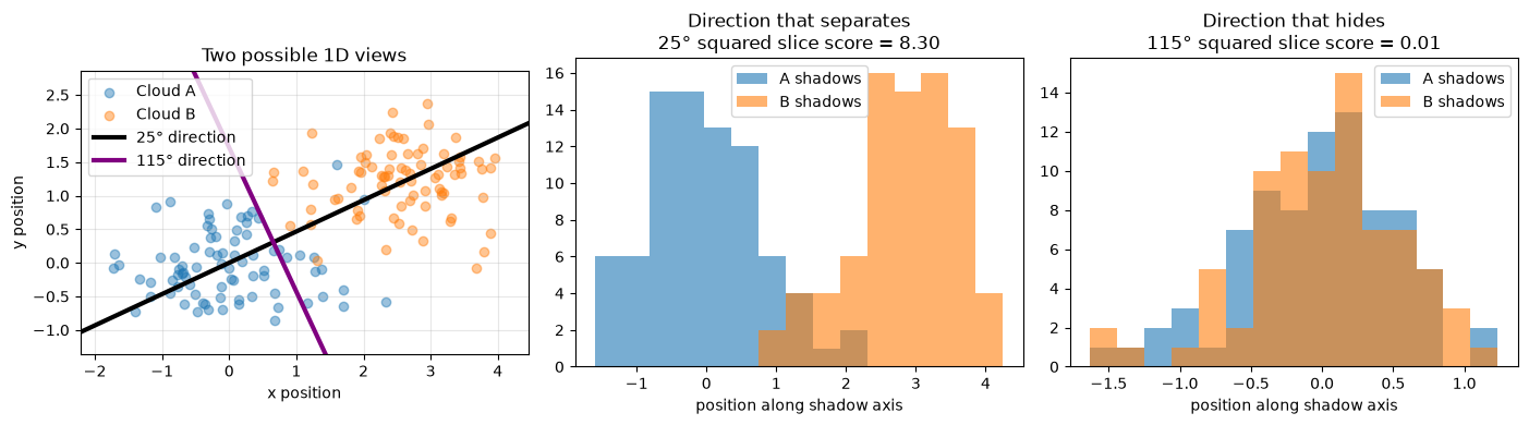
That is why sliced-Wasserstein does not trust just one projection. It samples many random directions, computes the simple 1D Wasserstein comparison for each one, and then averages the results.
In the plot below, we estimate the squared 2-sliced-Wasserstein distance, written (SW_2^2). With only a few slices, the estimate jumps around because each new direction can change the average a lot. But as more directions are included, the running average converges to a stable result.
max_views = 500
dirs = rng.normal(size=(max_views, 2))
dirs = dirs / np.linalg.norm(dirs, axis=1, keepdims=True)

scores = []
for v in dirs:
    a, b = cloud_A @ v, cloud_B @ v
    scores.append(np.mean((np.sort(a) - np.sort(b))**2))

running_avg = np.cumsum(scores) / np.arange(1, max_views + 1)

plt.figure(figsize=(8, 4))
plt.plot(np.arange(1, max_views + 1), running_avg)
plt.xlabel("number of directions / views")
plt.ylabel("running average SW₂² estimate")
plt.title("Squared sliced-Wasserstein estimate stabilises as views increase")
plt.grid(alpha=0.3);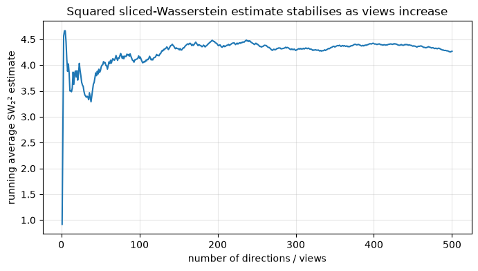
The curve shows the running average of the slice scores. Early on, each new direction can move the estimate a lot. After many directions, each extra slice has less influence, so the estimate becomes steadier.
This is the practical tradeoff behind SWD. More slices give a better picture of the full cloud, but they cost more computation. VISReg uses this idea in high-dimensional embedding space: instead of directly comparing two complicated clouds, it compares many cheap 1D shadows and averages the result.
A Gaussian-like cloud vs a collapsed cloud
Now we can use sliced-Wasserstein distance as a diagnostic for an embedding cloud.
In a self-supervised model, each image becomes a point in embedding space. If training goes wrong, those points can collapse almost into a single spot, or stretch along one narrow direction. Both cases throw away useful information. A Gaussian-like cloud is centred, spread across dimensions, and closer in shape to the Gaussian reference that VISReg compares against.
Before comparing the toy clouds, we need a couple of small helper functions. sliced_wasserstein_sq repeats the slicing idea from the previous section: choose random directions, project both clouds onto each direction, sort the 1D shadows, compare them by rank, and average the squared differences. The helper can also accept a precomputed set of directions, which lets us compare several clouds using exactly the same slices.
def random_unit_dirs(dim, n_dirs):
    dirs = rng.normal(size=(n_dirs, dim)); dirs /= np.linalg.norm(dirs, axis=1, keepdims=True)
    return dirs

def sliced_wasserstein_sq(A, B, n_dirs=200, dirs=None):
    dirs = random_unit_dirs(A.shape[1], n_dirs) if dirs is None else dirs
    return np.mean([np.mean((np.sort(A @ v) - np.sort(B @ v))**2) for v in dirs])
Next we create three toy embedding clouds. The Gaussian-like cloud is drawn from a normal distribution, so it should look similar to the Gaussian target. The collapsed cloud has almost no spread. The skinny cloud still varies in one direction, but is squeezed tightly in the other.
For these toy visuals, the Gaussian target is another sampled point cloud. In VISReg itself, the reference shadows are sorted Gaussian quantiles, but the intuition is the same: compare the embedding cloud against a Gaussian-shaped reference.
A Gaussian quantile is a reference position from a normal distribution. For example, the 50% quantile is the middle of the Gaussian, while the 95% quantile is far out in the right tail. Using sorted Gaussian quantiles gives a clean idealized 1D Gaussian reference to compare against, instead of sampling a noisy random target cloud.
n = 200
gaussian_like = rng.normal(0, 1, size=(n, 2))
collapsed = rng.normal(0, 0.05, size=(n, 2))
skinny = np.c_[rng.normal(0, 1.5, n), rng.normal(0, 0.08, n)]
target = rng.normal(0, 1, size=(n, 2))
# Toy approximation: VISReg uses sorted Gaussian quantiles; here we use sampled Gaussian points for visual comparison.
fig, axes = plt.subplots(1, 3, figsize=(11, 3.2), sharex=True, sharey=True)
for ax, pts, title in zip(axes, [gaussian_like, collapsed, skinny], ["Gaussian-like", "collapsed", "skinny"]):
ax.scatter(pts[:,0], pts[:,1], alpha=0.55)
ax.set_title(title); ax.set_aspect("equal"); ax.grid(alpha=0.3)
plt.suptitle("Three possible embedding-cloud shapes");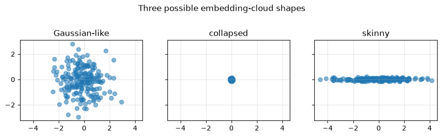
The plot makes the cloud shapes easy to see, but the table below gives us a numerical sanity check. We compare each cloud to a Gaussian target using the squared sliced-Wasserstein estimate, and also show the standard deviation along x and y so we can see how spread out each cloud is.
To make the three scores comparable, we use the same 200 random slice directions for every cloud. Each score is the average squared 1D Wasserstein value over those shared directions.
swd_dirs = random_unit_dirs(2, 200)
pd.DataFrame({
    "cloud": ["Gaussian-like", "collapsed", "skinny"],
    "SW₂² to Gaussian target": [sliced_wasserstein_sq(gaussian_like, target, dirs=swd_dirs), sliced_wasserstein_sq(collapsed, target, dirs=swd_dirs), sliced_wasserstein_sq(skinny, target, dirs=swd_dirs)],
    "x spread": [gaussian_like[:,0].std(), collapsed[:,0].std(), skinny[:,0].std()],
    "y spread": [gaussian_like[:,1].std(), collapsed[:,1].std(), skinny[:,1].std()],
}).round(3)| cloud | SW₂² to Gaussian target | x spread | y spread | |
|---|---|---|---|---|
| 0 | Gaussian-like | 0.040 | 1.002 | 1.032 |
| 1 | collapsed | 0.937 | 0.046 | 0.050 |
| 2 | skinny | 0.291 | 1.662 | 0.081 |
Reading this experiment
The Gaussian-like cloud has the smallest squared sliced-Wasserstein estimate to the Gaussian target. That is what we would hope to see: its spread is close to 1 in both directions, and its overall shape is similar to the target.
The collapsed cloud has the largest squared estimate. Its x and y spreads are both close to 0, so almost all points have fallen into one tiny region. This is exactly the kind of representation collapse that a regularizer should penalize.
The skinny cloud sits in between. It has plenty of spread in the x direction, but almost no spread in the y direction. So it has not fully collapsed, but it is still very non-Gaussian: most of the variation lives along one narrow axis.
This is the useful behaviour of the squared sliced-Wasserstein estimate here. It does not just check whether the embeddings have a nonzero variance somewhere. It compares the overall shape of the embedding cloud to a reference Gaussian cloud, so collapse and anisotropic “skinny” structure both receive larger penalties than the Gaussian-like case.
What sliced-Wasserstein sees in each cloud
The previous section showed that the Gaussian-like, collapsed, and skinny clouds receive very different squared sliced-Wasserstein scores. Now let’s look inside that calculation.
For each cloud, SWD does not compare the 2D scatter plot directly. It repeatedly projects the cloud and the Gaussian reference onto 1D lines, then compares those projected shadows by sorting and matching ranks.
The plots below show one such random projection. They help explain why collapse and skinny anisotropic structure receive larger penalties than the Gaussian-like cloud.
clouds = {"Gaussian-like": gaussian_like, "collapsed": collapsed, "skinny": skinny}
v = rng.normal(size=2); v = v / np.linalg.norm(v)
fig, axes = plt.subplots(1, 3, figsize=(12, 3.6), sharex=True, sharey=True)
for ax, (name, pts) in zip(axes, clouds.items()):
    ax.scatter(target[:,0], target[:,1], s=18, alpha=0.25, label="ideal Gaussian", color="gray")
    ax.scatter(pts[:,0], pts[:,1], s=22, alpha=0.65, label=name)
    axis_t = np.array([-4, 4])
    axis_pts = axis_t[:, None] * v
    ax.plot(axis_pts[:,0], axis_pts[:,1], color="black", lw=2, label="shadow direction")
    ax.set_title(name, pad=12); ax.set_aspect("equal"); ax.grid(alpha=0.3); ax.legend()
plt.suptitle("Each input cloud overlaid on the ideal Gaussian reference", y=1.08);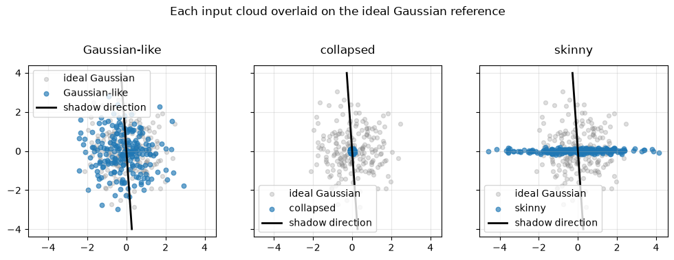
Shadows: what sliced-Wasserstein actually compares
The scatter plots above show the original 2D clouds, but sliced-Wasserstein does not compare those pictures directly. For each random direction, it turns both the input cloud and the Gaussian reference into 1D shadow samples, then sorts those shadows and compares them rank by rank.
The plots below show those 1D shadows for the same direction. This is the level at which the squared slice score is actually computed.
fig, axes = plt.subplots(1, 3, figsize=(12, 3.4), sharey=True)
for ax, (name, pts) in zip(axes, clouds.items()):
    ax.hist(target @ v, bins=20, alpha=0.45, label="ideal Gaussian", color="gray")
    ax.hist(pts @ v, bins=20, alpha=0.65, label=name)
    ax.set_title(f"{name}: one shadow view", pad=12); ax.grid(alpha=0.3); ax.legend()
plt.suptitle("Projected shadows along the same random direction", y=1.08);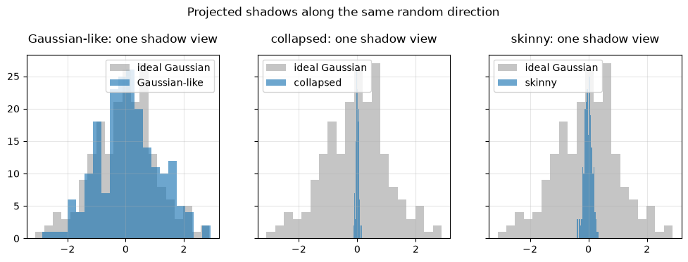
Reading these visuals
Each panel shows one random 1D projection of an input cloud compared with the same ideal Gaussian reference.
For the Gaussian-like cloud, the blue and grey histograms overlap fairly well. They are not identical, because both clouds are finite random samples, but their centres and spreads are similar. This is why its sliced-Wasserstein distance to the target was small.
For the collapsed cloud, the blue histogram is squeezed into a very narrow spike near zero. The Gaussian reference has much wider shadows, so the sorted 1D values are far apart for most ranks. This produces a large penalty: the representation has lost almost all variation.
For the skinny cloud, this single shadow view can be more subtle. Along some directions the skinny cloud may look reasonably spread out, while along directions nearly perpendicular to its long axis it will look almost collapsed. Averaging many shadow comparisons is what lets sliced-Wasserstein detect this anisotropic shape rather than being fooled by one lucky view.
What SWD can see: same spread, different shape
Now we isolate one of the reasons SWD is useful as a shape comparison. So far, the examples have mostly involved clouds that are shifted, collapsed, or stretched. Those differences are fairly easy to spot from the mean and spread. But distributions can also differ in a more subtle way: they can have similar centres and similar x/y spreads, while still having very different shapes.
To make that concrete, we will compare two clouds:
- A normal Gaussian blob.
- A ring-shaped cloud.
Both are centred near zero, and both spread out by about the same amount in the x and y directions. A small table of means and standard deviations will therefore make them look fairly similar. But visually they are not similar at all. The blob fills the middle; the ring leaves a hole.
This is exactly the kind of difference we want a distribution-shape regularizer to notice.
n = 400
blob = rng.normal(0, 1, size=(n, 2))
angles = rng.uniform(0, 2*np.pi, n)
ring = np.sqrt(2) * np.c_[np.cos(angles), np.sin(angles)] + rng.normal(0, 0.08, size=(n, 2))
target = rng.normal(0, 1, size=(n, 2))
fig, axes = plt.subplots(1, 2, figsize=(8, 3.5), sharex=True, sharey=True)
for ax, pts, title in zip(axes, [blob, ring], ["Gaussian blob", "Ring cloud"]):
ax.scatter(pts[:,0], pts[:,1], s=14, alpha=0.55)
ax.set_title(title); ax.set_aspect("equal"); ax.grid(alpha=0.3)
plt.suptitle("Similar centre/spread, different shape");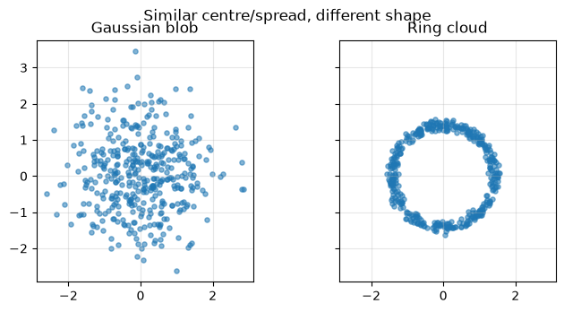
The plot makes the difference obvious: the Gaussian blob puts many points near the centre, while the ring keeps most points at a roughly fixed radius. Next we’ll check why simple mean and standard-deviation summaries can miss that difference.
swd_dirs = random_unit_dirs(2, 200)
pd.DataFrame({
    "cloud": ["blob", "ring"],
    "mean x": [blob[:,0].mean(), ring[:,0].mean()],
    "mean y": [blob[:,1].mean(), ring[:,1].mean()],
    "std x": [blob[:,0].std(), ring[:,0].std()],
    "std y": [blob[:,1].std(), ring[:,1].std()],
    "SW₂² to Gaussian target": [sliced_wasserstein_sq(blob, target, dirs=swd_dirs), sliced_wasserstein_sq(ring, target, dirs=swd_dirs)],
}).round(3)| cloud | mean x | mean y | std x | std y | SW₂² to Gaussian target | |
|---|---|---|---|---|---|---|
| 0 | blob | -0.009 | 0.056 | 0.956 | 1.020 | 0.018 |
| 1 | ring | 0.009 | 0.084 | 0.985 | 1.021 | 0.119 |
SWD makes that mismatch visible after projection. Along many random lines, the ring’s shadows do not look quite like Gaussian shadows: too much mass sits away from the centre, and too little sits near the middle. The mismatch is picked up by sorting the shadow values and comparing them by rank against shadows from a Gaussian target.
This is an important part of the VISReg story. VISReg is not only asking whether the embedding cloud has enough spread. It is also asking whether the cloud has the right distributional shape. That makes it stronger than checks based only on variance or covariance.
A VISReg/SIGReg comparison
SIGReg and VISReg are closely related because both use random 1D sketches to control the shape of the embedding distribution.
SIGReg’s idea is direct: make the embedding cloud look like an isotropic Gaussian, (N(0, I)). It asks the cloud’s random shadows to look like Gaussian shadows. That is a strong distributional target: it encourages the representation to be centred, spread out, and Gaussian-shaped.
VISReg keeps that sketching idea, but separates the tasks more explicitly. Its variance term controls the overall scale of the embedding cloud, while its sliced-Wasserstein/sketching term focuses on distributional shape. In other words, VISReg does not ask one objective to handle scale and shape at the same time.
This separation is the main conceptual difference:
| method | main idea | possible limitation |
|---|---|---|
| SIGReg | align embeddings directly to an isotropic Gaussian | scale and shape are tied together |
| VISReg | use variance for scale, SWD/sketching for shape | a little more structured, but more flexible |
So in the toy examples above, SIGReg is like saying: “make the whole blue cloud look like the grey Gaussian.” VISReg is more like saying: “first make sure the cloud has enough spread, then make its normalized shape look Gaussian.”
That is why sliced-Wasserstein distance is central to VISReg. It gives a cheap way to compare high-dimensional embedding clouds against a Gaussian-shaped target, while still detecting problems like collapse, skinny anisotropic structure, or non-Gaussian shapes such as the ring example.
Why the ring gets caught: look at the shadows
The ring and the blob have similar means and similar spreads, so a basic summary table makes them look almost the same.
SWD asks a more detailed question: when we project the points onto a line, does the whole 1D shadow look Gaussian?
For a Gaussian blob, most projected views are still Gaussian-like: thick near the middle, thinner toward the tails. A ring behaves differently. In many directions, points from the two sides of the ring land away from the centre, leaving less mass near zero. The hollow middle is no longer visible as a hole, but it still leaves a pattern in the shadow.
v = np.array([1.0, 0.0])
blob_shadow = blob @ v
ring_shadow = ring @ v
target_shadow = target @ vplt.figure(figsize=(8, 3.5))
plt.hist(target_shadow, bins=30, alpha=0.35, label="Gaussian target", color="gray")
plt.hist(blob_shadow, bins=30, alpha=0.55, label="Blob shadow")
plt.hist(ring_shadow, bins=30, alpha=0.55, label="Ring shadow")
plt.title("One shadow direction: blob vs ring")
plt.xlabel("position along shadow line")
plt.ylabel("count")
plt.legend()
plt.grid(alpha=0.3);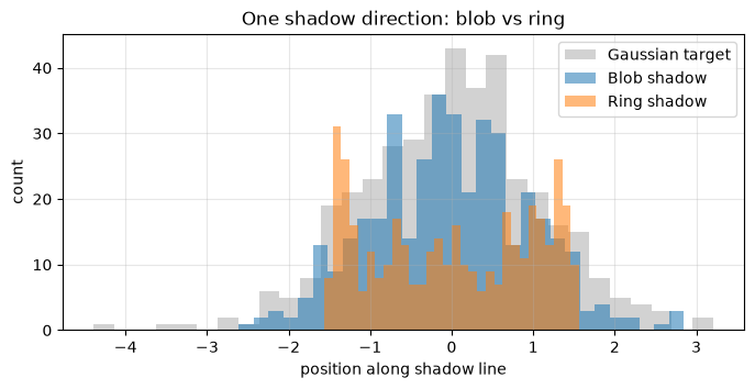
pd.DataFrame({
    "shadow": ["target", "blob", "ring"],
    "mean": [target_shadow.mean(), blob_shadow.mean(), ring_shadow.mean()],
    "std": [target_shadow.std(), blob_shadow.std(), ring_shadow.std()],
    "middle gap: fraction near 0": [
        np.mean(np.abs(target_shadow) < 0.25),
        np.mean(np.abs(blob_shadow) < 0.25),
        np.mean(np.abs(ring_shadow) < 0.25),
    ],
}).round(3)| shadow | mean | std | middle gap: fraction near 0 | |
|---|---|---|---|---|
| 0 | target | -0.012 | 1.094 | 0.215 |
| 1 | blob | -0.009 | 0.956 | 0.205 |
| 2 | ring | 0.009 | 0.985 | 0.148 |
The histogram shows the shape mismatch in one slice. The Gaussian target and the blob both put a reasonable amount of mass near zero. The ring puts less mass there, because many of its points come from the outer band of the circle.
The table makes this precise. All three shadows have similar means and standard deviations, so those two statistics do not expose the ring very clearly. But the fraction of values close to zero is much smaller for the ring: 0.148, compared with 0.215 for the Gaussian target and 0.205 for the blob.
This is what SWD picks up. It not only asks how wide the cloud is. It compares the sorted shadow values, so differences in the full 1D shape affect the score. One shadow gives a clue; many random shadows make the hollow-ring structure hard to hide.
From a few slices to a stable SWD estimate
We have already seen that one projection can mislead. Now we can ask a harder question: does the blob-vs-ring difference survive when we average many random projections?
This matters because the ring has similar mean and coordinate-wise spread to the Gaussian blob. If squared SWD is really detecting distributional shape, the ring should stay farther from the Gaussian target even after the estimate stabilizes. The table below compares the two clouds using different numbers of directions; for each row, the blob and ring are evaluated with the same sampled directions.
rows = []
for k in [5, 20, 100, 500]:
    swd_dirs = random_unit_dirs(2, k)
    rows.append({
        "directions": k,
        "blob to Gaussian": sliced_wasserstein_sq(blob, target, dirs=swd_dirs),
        "ring to Gaussian": sliced_wasserstein_sq(ring, target, dirs=swd_dirs),
    })
pd.DataFrame(rows).round(4)| directions | blob to Gaussian | ring to Gaussian | |
|---|---|---|---|
| 0 | 5 | 0.0175 | 0.1114 |
| 1 | 20 | 0.0156 | 0.1143 |
| 2 | 100 | 0.0196 | 0.1249 |
| 3 | 500 | 0.0176 | 0.1188 |
The exact values move around because the projection directions are sampled randomly.
The important part is the pattern. The blob stays close to the Gaussian target, while the ring stays noticeably farther away. Even though the ring has similar mean and spread, its projected shadows have the wrong shape often enough that SWD gives it a larger score.
max_views = 500
dirs = rng.normal(size=(max_views, 2))
dirs = dirs / np.linalg.norm(dirs, axis=1, keepdims=True)

blob_slice_scores = []
ring_slice_scores = []
for v in dirs:
    blob_slice_scores.append(np.mean((np.sort(blob @ v) - np.sort(target @ v))**2))
    ring_slice_scores.append(np.mean((np.sort(ring @ v) - np.sort(target @ v))**2))

views = np.arange(1, max_views + 1)
blob_running = np.cumsum(blob_slice_scores) / views
ring_running = np.cumsum(ring_slice_scores) / views

plt.figure(figsize=(8, 4))
plt.plot(views, blob_running, label="blob to Gaussian")
plt.plot(views, ring_running, label="ring to Gaussian")
plt.xlabel("number of directions / views")
plt.ylabel("running average SW₂² estimate")
plt.title("Running squared SWD estimate as views increase")
plt.legend()
plt.grid(alpha=0.3);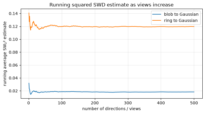
The running-average plot shows the same idea more clearly. Early estimates wobble because each new direction has a large effect on the average. After enough directions, the curves settle.
The ring remains well above the blob, which is the point of this example: SWD is not just checking centre and spread. By comparing many 1D shadows, it can detect distribution-shape differences that simple summary statistics miss.
Where SWD fits inside the VISReg loss
VISReg uses sliced-Wasserstein distance as one part of its representation-learning objective.
During training, each image is augmented into different views. The model should map matching views close together, so the representation keeps information that is stable across augmentations. But this alone can lead to collapse: the model could map many images to almost the same vector and still make matching views close.
VISReg avoids this with three regularization ideas:
- A scale term keeps the embedding cloud spread out
- A center term keeps it near the origin
- And the sliced-Wasserstein shape term checks whether the normalized cloud looks like samples from an isotropic Gaussian.
The equations below show where that shape-checking term sits inside the full loss, according to the VISReg paper.
The regularization details here are included for completeness, rather than as a full derivation. A future post will hopefully go through the VISReg objective more carefully. Here, the goal is just to show where SWD sits inside the overall loss. The equations below follow the paper’s structure but use slightly simplified notation; averaging constants are written explicitly where they help the intuition.
\[ \mathcal L_{\mathrm{VISReg}}=(1-\lambda)\,\mathcal L_{\mathrm{pred}}+\lambda\,\mathcal L_{\mathrm{Reg}} \]
The prediction term, \(\mathcal L_{\mathrm{pred}}\), is the “match related views” part. If two crops or augmentations come from the same image, their embeddings should be compatible.
The regularization term, \(\mathcal L_{\mathrm{Reg}}\), looks at the batch as a whole. It is less concerned with which image produced which vector, and more concerned with the shape of the full embedding cloud.
VISReg splits this regularization into three pieces:
\[ \mathcal L_{\mathrm{Reg}} = \lambda_{\mathrm{scale}}\mathcal L_{\mathrm{scale}} + \lambda_{\mathrm{shape}}\mathcal L_{\mathrm{shape}} + \lambda_{\mathrm{center}}\mathcal L_{\mathrm{center}} \]
Each piece has a different job. The scale term checks that each embedding dimension has enough spread. The center term keeps the batch mean near zero. The shape term is where sliced-Wasserstein distance enters.
The scale term is:
\[ \mathcal L_{\mathrm{scale}}=\frac{1}{D}\sum_{j=1}^{D}\left(1-\sigma_j(\hat Z)\right)^2 \]
Here, \(\sigma_j(\hat Z)\) is the standard deviation of the centred embeddings along dimension \(j\). If a dimension collapses and has almost no variation, this term pushes it back toward unit spread.
Before the shape check, VISReg normalizes the centred embeddings:
\[ \tilde Z = \frac{\hat Z}{\mathrm{sg}(\sigma)+\epsilon} \]
The sg means stop-gradient. In plain terms, the shape loss is allowed to look at the measured scale, but not change it directly. That keeps the two jobs separate: scale controls how large the cloud is, while shape checks what the normalized cloud looks like.
The shape term is the sliced-Wasserstein part:
\[ \mathcal L_{\mathrm{shape}} = \frac{1}{K}\sum_{k=1}^{K} \mathrm{mean}\left( \left( \mathrm{sort}(\tilde Z w_k)-q_{\mathcal N} \right)^2 \right) \]
This is the same slicing idea we built up visually. For each random direction \(w_k\), VISReg projects the normalized embedding cloud onto a line. It sorts those projected values and compares them with sorted reference values from a standard Gaussian.
So \(\mathcal L_{\mathrm{shape}}\) asks: after centering and scale-normalizing the batch, do its 1D shadows look Gaussian-like?
The center term is simpler:
\[ \mathcal L_{\mathrm{center}}=\mathrm{mean}(\mu^2) \]
It keeps the batch mean close to zero, so the cloud does not drift away from the origin.
The two sets of lambda’s have different roles. The outer \(\lambda\) controls the balance between prediction and regularization. It is used like a 0 to 1 blend:
\[ (1-\lambda)\,\mathcal L_{\mathrm{pred}} + \lambda\,\mathcal L_{\mathrm{Reg}} \]
The inner lambda’s, \(\lambda_{\mathrm{scale}}\), \(\lambda_{\mathrm{shape}}\), and \(\lambda_{\mathrm{center}}\), control the relative strength of the three regularization pieces. In the VISReg paper’s ablations, these three weights are kept normalised so that:
\[ \lambda_{\mathrm{scale}}+\lambda_{\mathrm{shape}}+\lambda_{\mathrm{center}}=3 \]
The default is (1, 1, 1). A shape-heavy setting such as (0.75, 1.5, 0.75) gives the SWD term more influence while keeping the total inner regularization weight fixed.
In summary, VISReg still learns by matching related image views, but SWD is the part of the regularizer that checks whether the embedding cloud has the right distributional shape.
Plain-English guide to the regularization terms
A useful way to read VISReg is that each term guards against a different failure mode.
The prediction term says: matching views of the same image should agree. This is the representation-learning part of the loss. But by itself, this does not prevent collapse, because a model could make every image look the same and still make matching views agree.
The center term says: keep the whole cloud near the origin. Without this, the embeddings could drift away even if their relative shape looked reasonable.
The scale term says: keep every dimension alive. If one embedding dimension has almost no variation across the batch, then that dimension is not carrying much information. Pushing each standard deviation toward 1 helps prevent the cloud from shrinking or losing dimensions.
The shape term says: after centering and scale-normalizing, the cloud should look Gaussian-like. This is where sliced-Wasserstein distance is used. It checks many 1D shadows of the embedding cloud and compares them with Gaussian shadows.
So the three regularization pieces can be read like this:
| term | plain-English job | failure it catches |
|---|---|---|
| center | keep the cloud near zero | drifting away from the origin |
| scale | keep dimensions spread out | collapse or dead dimensions |
| shape / SWD | make the normalized cloud Gaussian-like | skinny, distorted, or non-Gaussian shapes |
The stop-gradient in the normalization step is important because it keeps these jobs separated. The shape loss sees the measured scale, but it does not directly control it. Scale is handled by the scale term; shape is handled by the sliced-Wasserstein term.
This separation is what makes VISReg conceptually more flexible than SIGReg. Instead of using one regularizer to do everything, it splits the problem into centre, scale, and shape. Sliced-Wasserstein distance is the shape-checking tool: it asks whether the embedding cloud has the right distributional form once the simpler centre and scale issues have been accounted for.
What we learned about Sliced-Wasserstein Distance
Sliced-Wasserstein Distance compares point clouds by turning a hard high-dimensional matching problem into many easy 1D ones. In this post, the reported values are squared estimates: for each random direction, we project both clouds onto a line, sort the shadow values, match by rank, and average the squared differences.
A single shadow can miss structure, but many random shadows make differences harder to hide. That is why SWD can catch not only collapse or anisotropy, but subtler shape differences such as the blob-vs-ring example, where simple means and standard deviations looked similar.
In VISReg, the point cloud is a batch of neural-network embeddings. The scale and center terms keep the cloud spread out and near zero, while the squared SWD shape term asks whether the normalized embeddings look Gaussian-like when viewed through many random projections.
Community
Explore together.
Share what you’re learning, ask questions, and swap ideas.
Join the ExploringML Discord.